Part 11: Static Magnetic Field

1. Biot-Savart Law

$$ d\vec{B} = \frac{\mu_0}{4\pi} \frac{I d\vec{l} \times \hat{r}}{r^2}, \quad \vec{B} = \int d\vec{B} $$

2. Gauss's Law & Ampere's Circuital Law

Gauss's Law for Magnetism: $\oint_S \vec{B} \cdot d\vec{S} = 0$
Ampere's Circuital Law: $\oint_L \vec{B} \cdot d\vec{l} = \mu_0 \sum I$

3. Typical Current-Carrying Magnetic Fields

① Infinite and Finite Wire:

Infinite Wire (Current $I$): $$ B \cdot 2\pi r = \mu_0 I \implies B = \frac{\mu_0 I}{2\pi r} $$
Finite Wire (Current $I$): 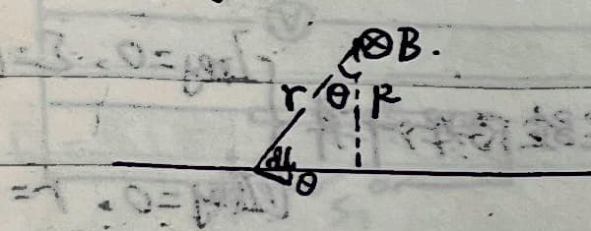$$ dB = \frac{\mu_0}{4\pi} \frac{I dl \cos\theta}{r^2} = \frac{\mu_0}{4\pi} \frac{I \cdot \left(\frac{R}{\cos^2\theta} d\theta\right) \cos\theta}{\left(\frac{R}{\cos\theta}\right)^2} = \frac{\mu_0 I \cos\theta d\theta}{4\pi R} $$

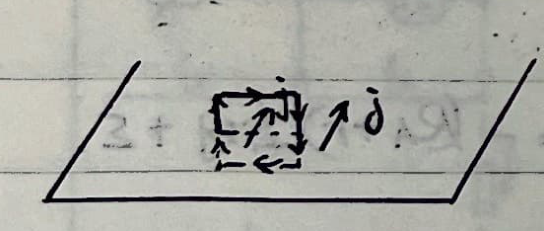
② Infinite Wide Flat Plate (Current density $j$):

$$ 2 B L = \mu_0 j L \implies B = \frac{1}{2} \mu_0 j $$

③ Infinite Cylindrical Surface: (Radius $R$, uniform current $I$ on surface)

$$ \begin{cases} r \ge R: & B \cdot 2\pi r = \mu_0 I \implies B = \frac{\mu_0 I}{2\pi r} \\ r < R: & B = 0 \end{cases} $$

④ Current-Carrying Ring:

$$ dB = \frac{\mu_0}{4\pi} \frac{I dl}{r^2} = \frac{\mu_0}{4\pi} \frac{I \cdot R d\theta}{r^2} $$ $$ \therefore B_{\perp} = 0, \quad B_{||} = \frac{\mu_0}{4\pi} \left( \frac{2\pi R I}{r^2} \frac{R}{r} \right) = \frac{\mu_0 R^2 I}{2r^3} $$

When $r = R$ (at the center), $B = \frac{\mu_0 I}{2R}$.

⑤ Current-Carrying Solenoid: (Turns per unit length $n$, total turns $N$, current per turn $I$)

$$ dl = n I dl \implies dB = \frac{\mu_0 R^2 n I dl}{2 r^3} $$ $$ \text{Also, } dl = \frac{r d\theta}{\sin\theta} \text{ and } r = \frac{R}{\sin\theta} $$ $$ \therefore dB = \frac{\mu_0 n I}{2} \sin\theta d\theta \implies B = \frac{\mu_0 n I}{2} (\cos\theta_2 - \cos\theta_1) $$

When the tube is infinitely long, $B = \mu_0 n I$.

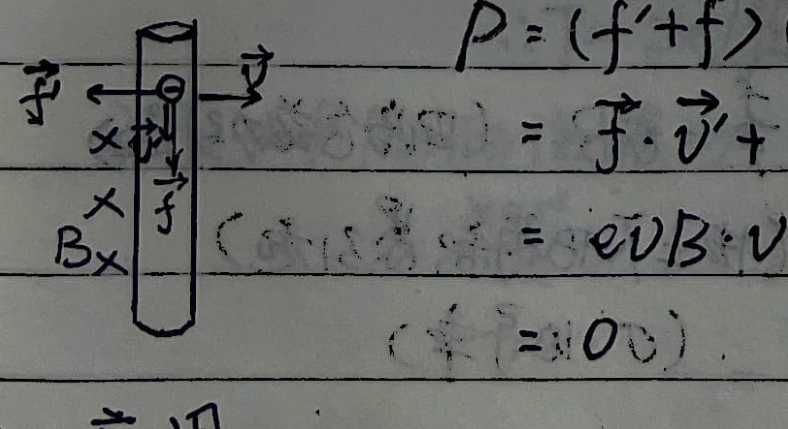
4. Lorentz Force

$$ \vec{F} = q \vec{v} \times \vec{B} $$

For a segment of conductive wire:

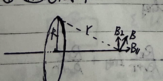
$$ d\vec{F} = dq \vec{v} \times \vec{B} = n S e dl \cdot \vec{v} \times \vec{B} = n S e v \cdot d\vec{l} \times \vec{B} = I d\vec{l} \times \vec{B} $$ $$ \therefore \vec{F} = \int I d\vec{l} \times \vec{B} \quad \text{— Ampere's Force} $$

① Ampere's Force Torque:

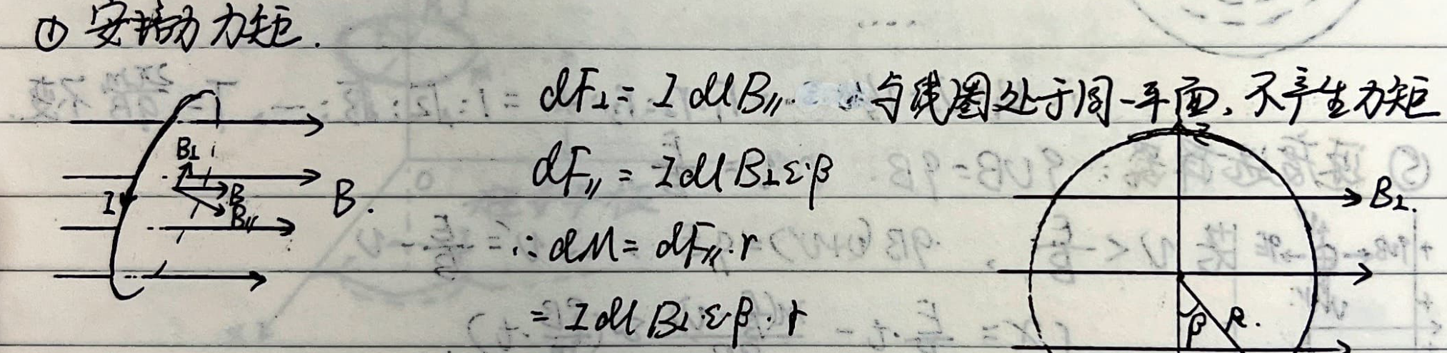$$ dF_{\perp} = I dl B_{\parallel} \quad \text{(In the same plane as the coil, produces no torque)} $$ $$ dF_{\parallel} = I dl B \sin\beta $$ $$ \therefore dM = dF_{\parallel} \cdot r = I dl B \sin\beta \cdot r = I \cdot R d\beta \cdot B \sin\beta \cdot R \sin\beta $$ $$ \therefore M = I R^2 B_{\perp} \int_0^{\pi} \sin^2\beta d\beta = \pi I R^2 B_{\perp} $$

Written in vector form: $\vec{M} = I \vec{S} \times \vec{B}$.

Defining magnetic moment: $\vec{m} = I \vec{S}$.

$$ \therefore \vec{M} = \vec{m} \times \vec{B} $$

② Lorentz Force Does No Work:

$$ P = \vec{F} \cdot \vec{v} = (q \vec{v} \times \vec{B}) \cdot \vec{v} = 0 $$

As electrons move with the conductor in a magnetic field at velocity $\vec{v}$, they experience a Lorentz force along the wire, gaining velocity $\vec{v}'$.

$$ P = (\vec{f}' + \vec{f}) \cdot (\vec{v} + \vec{v}') = \vec{f} \cdot \vec{v}' + \vec{f}' \cdot \vec{v} = e v B \cdot v' - e v' B \cdot v = 0 $$

5. Applications

① Hall Effect:

$$ e E_H = e v B \implies U_H = E_H h = v B h $$ $$ \text{Also } I = n b h q v \implies v = \frac{I}{n b h q} \quad \therefore U_H = \frac{I B}{n q b} $$

Hall Resistance: $R_H = \frac{B}{n q b}$.

② Galvanometer/Ammeter: $B I S = k \theta$.

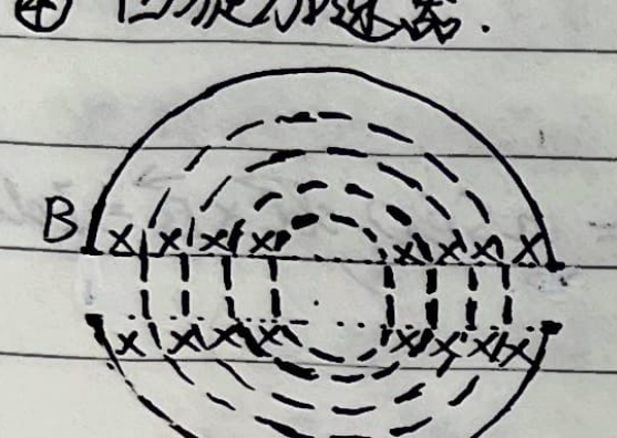
③ Mass Spectrometer:

$$ m \frac{v^2}{r} = q v B \implies r = \frac{m v}{q B}, \quad T = \frac{2\pi m}{q B} $$

④ Cyclotron:

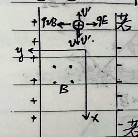
$$ q U = \frac{1}{2} m v_1^2 \implies r_1 = \frac{m v_1}{q B}, \quad v_1 = \sqrt{\frac{2 q U}{m}} $$ $$ q U = \frac{1}{2} m v_2^2 - \frac{1}{2} m v_1^2 \implies r_2 = \frac{m v_2}{q B}, \quad v_2 = \sqrt{\frac{4 q U}{m}} $$ $$ q U = \frac{1}{2} m v_3^2 - \frac{1}{2} m v_2^2 \implies r_3 = \frac{m v_3}{q B}, \quad v_3 = \sqrt{\frac{6 q U}{m}} $$ $$ \dots $$ $$ \therefore v_1 : v_2 : v_3 : \dots = r_1 : r_2 : r_3 : \dots = 1 : \sqrt{2} : \sqrt{3} : \dots $$

And the period $T = \frac{2\pi m}{q B}$ remains constant.

⑤ Velocity Selector: $q v B = q E \implies v = \frac{E}{B}$.

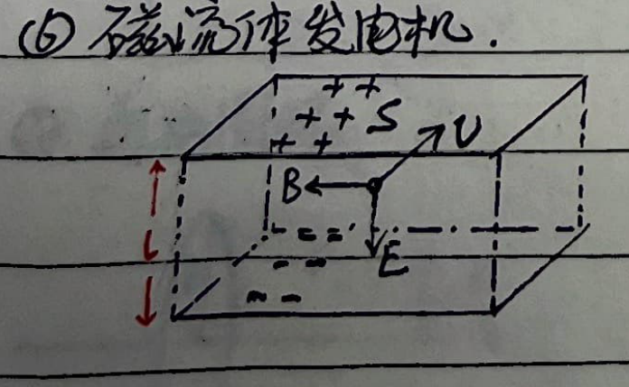
If $v < \frac{E}{B}$: $q B (v + v') = q E \implies v' = \frac{E}{B} - v$. $$ \begin{cases} x = \frac{E}{B} t - \frac{m (\frac{E}{B} - v)}{q B} \sin\left(\frac{q B}{m} t\right) \\ y = \frac{m (\frac{E}{B} - v)}{q B} \cos\left(\frac{q B}{m} t\right) - \frac{m (\frac{E}{B} - v)}{q B} \end{cases} $$
If $v > \frac{E}{B}$: $q B v = q E + q B v' \implies v' = v - \frac{E}{B}$. $$ \begin{cases} x = \frac{E}{B} t + \frac{m \left(v - \frac{E}{B}\right)}{q B} \sin\left(\frac{q B}{m} t\right) \\ y = \frac{m \left(v - \frac{E}{B}\right)}{q B} - \frac{m \left(v - \frac{E}{B}\right)}{q B} \cos\left(\frac{q B}{m} t\right) \end{cases} $$

⑥ Magnetohydrodynamic (MHD) Generator:

$$ \begin{cases} \text{Non-electrostatic force: } E_{ne} = \frac{F}{q} = v B \quad \text{(Caused by Lorentz force)} \\ \text{Electrostatic force: } E_s \quad \text{(Caused by charge accumulation)} \end{cases} $$ $$ \therefore I = \sigma (E_{ne} - E_s) \cdot S \quad (\text{where } \sigma \text{ is conductivity}) $$

Total power: $P = I E_{ne} l$.

Internal resistance power: $P_r = I (E_{ne} - E_s) l$.

Output power: $P_{\text{out}} = I E_s l = \sigma (v B - E_s) E_s V \le \frac{1}{4} \sigma v^2 B^2 V$ (where $V$ is the fluid volume between plates).

⑦ Electron Microscope:

Pitch: $h = v_{\parallel} T = \frac{2\pi m}{q B} v_{\parallel} \approx \frac{2\pi m}{q B} v$.

⑧ Magnetic Mirror:

$$ |\vec{m}| = I S = \frac{q}{T} \pi r^2 = \frac{q}{\frac{2\pi m}{q B}} \pi r^2 = \frac{q^2 B}{2 m} r^2 $$ $$ \text{Since } \frac{m v_{\perp}^2}{r} = q v_{\perp} B \implies r = \frac{m v_{\perp}}{q B} $$ $$ \therefore |\vec{m}| = \frac{m v_{\perp}^2}{2 B} $$

Due to the conservation of magnetic moment:

$$ \frac{m v_{\perp}^2}{2 B} = \frac{m v_0^2 \sin^2\theta}{2 B_0} = \frac{m v^2}{2 B} \implies \sin\theta_m = \sqrt{\frac{B_0}{B_m}} $$

⑨ Image Current: ($r \gg h$)

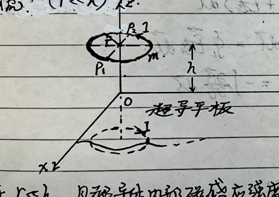
Since $r \gg h$, and the magnetic field inside the superconductor is zero, the magnetic field just outside the surface is parallel to the surface. This is equivalent to an image current at $z = -h$, with the two ring currents being anti-parallel.

$$ m g = \frac{\mu_0 I}{2\pi \cdot 2h} \cdot 2\pi r \cdot I \implies I = \sqrt{\frac{2 m g h}{\mu_0 r}} $$

If the ring oscillates slightly up and down: $$ F = \frac{\mu_0 r I^2}{2(h - x)} - m g \approx m g + \frac{\mu_0 r I^2}{2 h^2} x $$ $$ \therefore T = 2\pi \sqrt{\frac{m}{\frac{\mu_0 r I^2}{2h^2}}} = 2\pi \sqrt{\frac{h}{g}} $$
If it oscillates slightly around the axis $P_1 P_2$: $$ M \approx \frac{\mu_0 r I^2}{2} \left( \frac{1}{2h - r\theta} - \frac{1}{2h + r\theta} \right) \cdot r \approx \frac{\mu_0 r^3 I^2}{4 h^2} \theta = \frac{m g r^2}{2h} \theta $$ $$ \therefore T = 2\pi \sqrt{\frac{\frac{1}{2} m r^2}{\frac{m g r^2}{2h}}} = 2\pi \sqrt{\frac{h}{g}} $$

Special Topic: Magnetohydrodynamic (MHD) Generator

Model: The cross section is a rectangle, with tube length $l$, width $a$, and height $b$. The top and bottom sides are insulators, and the two sides separated by distance $a$ are conductors with negligible resistance, connected to a load $R_L$. The entire tube is in a region of uniform magnetic field, where $B$ is perpendicular to the top and bottom sides, pointing upwards. A plasma with resistivity $\rho$ flows through the tube along the $l$ direction at a uniform velocity. The frictional force it experiences is proportional to the flow velocity. A constant pressure difference $p$ is maintained at both ends of the tube. Without a magnetic field, the steady flow velocity of the plasma is $v_0$. What is the steady flow velocity when there is a magnetic field?

Without a magnetic field:

$$ \Delta F = p \cdot ab, \quad f_0 = k v_0 \quad \text{and} \quad \Delta F = f_0 \implies k = \frac{pab}{v_0} $$

With a magnetic field, the plasma is deflected by the Lorentz force and hits the side plates. At the same time, ions fly out to the other side plate, forming a circuit. The induced electromotive force is $\mathcal{E} = Bav$.

$$ \therefore I = \frac{\mathcal{E}}{R} = \frac{Bav}{R_L + \rho \frac{a}{bl}} $$ $$ \therefore \text{Ampere force } F = B I a = \frac{B^2 a^2 v}{R_L + \rho \frac{a}{bl}} $$

Also, $\Delta F = F + f$

$$ \implies pab = \frac{B^2 a^2 v}{R_L + \rho \frac{a}{bl}} + kv = \frac{B^2 a^2 v}{R_L + \rho \frac{a}{bl}} + pab \frac{v}{v_0} $$ $$ \therefore v = \frac{pab}{\frac{pab}{v_0} + \frac{B^2 a^2}{R_L + \rho \frac{a}{bl}}} $$ $$ \therefore \mathcal{E} = Bav = \frac{B a v_0}{1 + \frac{B^2 a l v_0}{p b \left(R_L + \rho \frac{a}{bl}\right)}} $$

Special Topic: Motion of Charged Particles in Special Electromagnetic Fields - Solving by Differential Equations

Problem: In space, establish a coordinate system as shown in the figure. A uniform electric field is along the positive x-axis, with magnitude $E$. A uniform magnetic field is at an angle $\alpha$ with the positive z-axis, with magnitude $B$. A particle of mass $m$ and charge $q$ ($q>0$) starts moving with an initial velocity $v_0$ along the positive y-axis. Find its equation of motion.

Set up the dynamic equations:

$$ \begin{cases} m a_x = qE + q v_y B_z \quad &(1) \\ m a_y = -q v_x B_z + q v_z B_x \quad &(2) \\ m a_z = -q v_y B_x \quad &(3) \end{cases} \implies \begin{cases} m v_x = q E t + q y B_z \quad &(4) \\ m (v_y - v_0) = -q x B_z + q z B_x \quad &(5) \\ m v_z = -q y B_x \quad &(6) \end{cases} $$

From (4) solve for $v_x$, from (6) solve for $v_z$, substitute both into (2), we get:

$$ m a_y = -q B_z \left(\frac{qE}{m}t + \frac{qB_z}{m}y\right) - \frac{q^2 B_x^2}{m} y = -\frac{q^2 E B_z}{m} t - \frac{q^2 B^2}{m} y $$

Rearranging terms gives:

$$ \frac{d^2 y}{dt^2} + \frac{q^2 E B_z}{m^2} t + \frac{q^2 B^2}{m^2} y = 0 \implies \frac{d^2 y}{dt^2} + \frac{q^2 B^2}{m^2} \left( \frac{E B_z}{B^2} t + y \right) = 0 $$

Since $\frac{d^2 y}{dt^2} = \frac{d^2}{dt^2}\left(y + \frac{E}{B}\cos\alpha \cdot t\right)$ and $\frac{B_z}{B} = \cos\alpha$, we get:

$$ \frac{d^2}{dt^2}\left(y + \frac{E}{B}\cos\alpha \cdot t\right) + \frac{q^2 B^2}{m^2} \left( y + \frac{E}{B}\cos\alpha \cdot t \right) = 0 \quad (7) $$

Solving yields: $y + \frac{E}{B}\cos\alpha \cdot t = A \sin\left(\frac{qB}{m} t + \theta\right)$.

At $t=0$, $y=0 \implies A\sin\theta = 0$.

$\frac{dy}{dt} = A \frac{qB}{m} \cos\left(\frac{qB}{m} t + \theta\right) - \frac{E}{B}\cos\alpha$. At $t=0$, $\frac{dy}{dt} = v_0$.

$$ \therefore \begin{cases} A\sin\theta = 0 \\ v_0 = \frac{qB}{m} A \cos\theta - \frac{E}{B}\cos\alpha \end{cases} \implies \begin{cases} \theta = 0 \\ A = \frac{m}{qB}\left(v_0 + \frac{E}{B}\cos\alpha\right) \end{cases} $$ $$ \therefore y = \frac{m}{qB}\left(v_0 + \frac{E}{B}\cos\alpha\right) \sin\left(\frac{qB}{m} t\right) - \frac{E}{B}\cos\alpha \cdot t \quad (10) $$

Substitute (10) into (4) to get:

$$ m \frac{dx}{dt} = qE \cdot t + q B \cos\alpha \left[ \frac{m}{qB}\left(v_0 + \frac{E}{B}\cos\alpha\right) \sin\left(\frac{qB}{m} t\right) - \frac{E}{B}\cos\alpha \cdot t \right] $$ $$ = qE \cdot t + m\left(v_0\cos\alpha + \frac{E}{B}\cos^2\alpha\right) \sin\left(\frac{qB}{m} t\right) - qE\cos^2\alpha \cdot t $$ $$ \therefore \frac{dx}{dt} = \left(v_0\cos\alpha + \frac{E}{B}\cos^2\alpha\right) \sin\left(\frac{qB}{m} t\right) + \frac{qE\sin^2\alpha}{m} \cdot t $$

Integrating gives $x$:

$$ \therefore x = \frac{m}{qB} \left(v_0\cos\alpha + \frac{E}{B}\cos^2\alpha\right) \left[1 - \cos\left(\frac{qB}{m} t\right)\right] + \frac{1}{2} \frac{qE\sin^2\alpha}{m} t^2 \quad (11) $$

Substitute (10) into (6) to get:

$$ m \frac{dz}{dt} = -q B \sin\alpha \left[ \frac{m}{qB}\left(v_0 + \frac{E}{B}\cos\alpha\right) \sin\left(\frac{qB}{m} t\right) - \frac{E}{B}\cos\alpha \cdot t \right] $$ $$ = -m\left(v_0\sin\alpha + \frac{E}{B}\sin\alpha\cos\alpha\right) \sin\left(\frac{qB}{m} t\right) + qE\sin\alpha\cos\alpha \cdot t $$ $$ \therefore \frac{dz}{dt} = -\left(v_0\sin\alpha + \frac{E}{B}\sin\alpha\cos\alpha\right) \sin\left(\frac{qB}{m} t\right) + \frac{qE\sin\alpha\cos\alpha}{m} \cdot t $$

Integrating gives $z$:

$$ \therefore z = -\frac{m}{qB} \left(v_0\sin\alpha + \frac{E}{B}\sin\alpha\cos\alpha\right) \left[1 - \cos\left(\frac{qB}{m} t\right)\right] + \frac{1}{2} \frac{qE\sin\alpha\cos\alpha}{m} t^2 \quad (12) $$