Part 8: Electrostatics

1. Electric Field Force

$$ \vec{F} = \frac{1}{4\pi\varepsilon_0} \frac{q_1 q_2}{r^2} \hat{r} $$

2. Electric Field Strength

$$ \vec{E} = \frac{\vec{F}}{q_0} $$ $$ \begin{cases} \vec{E} = \frac{1}{4\pi\varepsilon_0} \sum \frac{q_i}{r_i^2} \hat{r}_i \quad (\text{for discrete charge systems}) \\ \vec{E} = \int d\vec{E} \quad (\text{for continuous charged bodies}) \end{cases} $$

In Electrostatic Fields:

Gauss's Law: $\Phi_e = \oint \vec{E} \cdot d\vec{S} = \frac{q}{\varepsilon_0} \quad (q \text{ is the net charge enclosed by the Gaussian surface})$
Circuital Law: $\oint \vec{E} \cdot d\vec{l} = 0$

① Electric field distribution of a point charge:

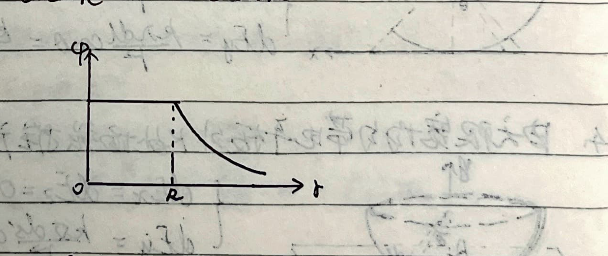
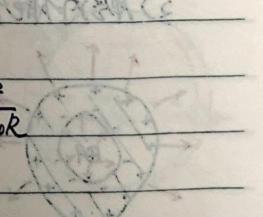
$$ E = \frac{1}{4\pi\varepsilon_0} \frac{Q}{r^2} $$

② Electric field distribution of a uniformly charged solid sphere (Charge volume density is equal everywhere, charges cannot move freely):

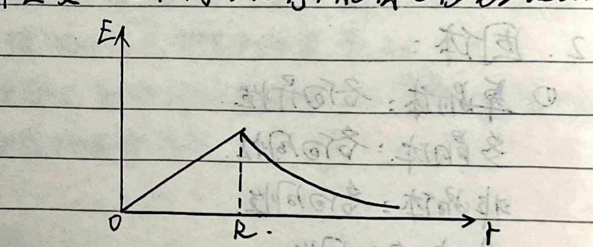
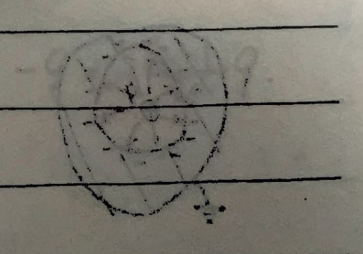
$$ \begin{cases} \text{When } r < R, \quad E \cdot 4\pi r^2 = \frac{1}{\varepsilon_0} \frac{r^3}{R^3} Q \\ \quad \therefore E = \frac{Q r}{4\pi\varepsilon_0 R^3} \\ \text{When } r \ge R, \quad E \cdot 4\pi r^2 = \frac{1}{\varepsilon_0} Q \\ \quad \therefore E = \frac{Q}{4\pi\varepsilon_0 r^2} \end{cases} $$ Electric field of solid sphere

③ Electric field distribution of a hollow spherical shell (Thin conducting spherical shell or solid conducting sphere, charges distribute on the outer surface due to electrostatic equilibrium, charges can move freely):

$$ \begin{cases} \text{When } r < R, \quad E \cdot 4\pi r^2 = 0 \\ \quad \therefore E = 0 \\ \text{When } r \ge R, \quad E \cdot 4\pi r^2 = \frac{1}{\varepsilon_0} Q \\ \quad \therefore E = \frac{Q}{4\pi\varepsilon_0 r^2} \end{cases} $$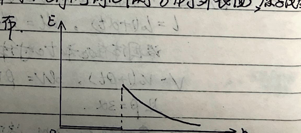 Electric field of hollow shell

④ Electric field distribution of an infinitely long conducting wire (Charge linear density $\lambda$):

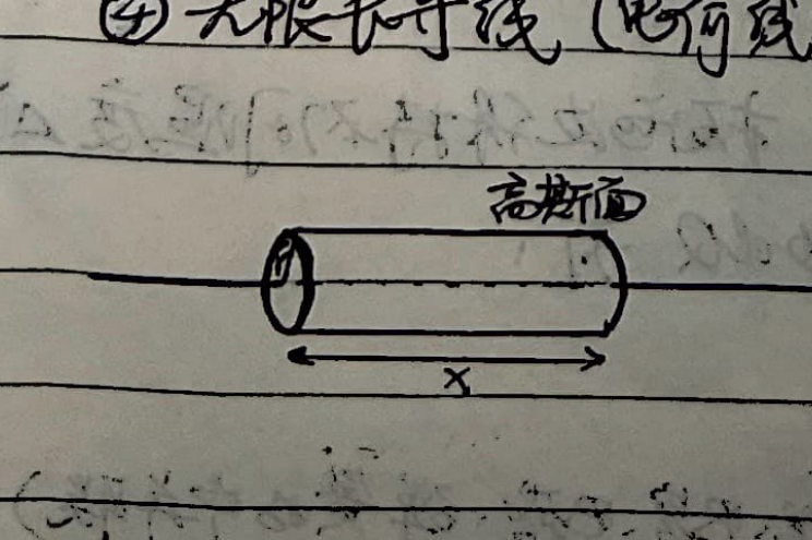
$$ E \cdot 2\pi r \cdot x = \frac{1}{\varepsilon_0} \lambda \cdot x $$ $$ \therefore E = \frac{\lambda}{2\pi\varepsilon_0 r} $$

⑤ Electric field distribution of an infinitely wide flat plate (Charge surface density $\sigma$):

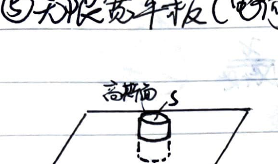
$$ 2E \cdot S = \frac{1}{\varepsilon_0} S \cdot \sigma $$ $$ \therefore E = \frac{\sigma}{2\varepsilon_0} $$

⑥ Surface of a conductor in electrostatic equilibrium:

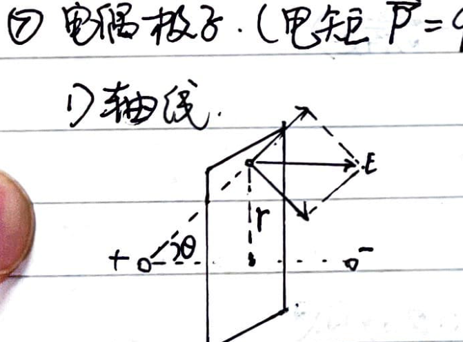
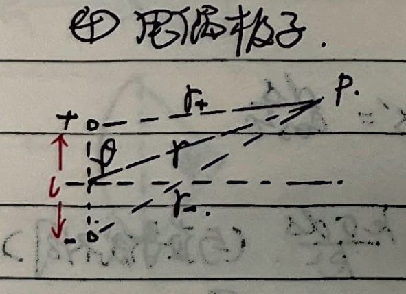
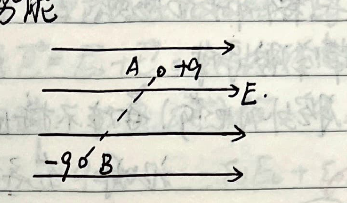
$$ E \cdot \Delta S = \frac{1}{\varepsilon_0} \Delta S \cdot \sigma $$ $$ \therefore E = \frac{\sigma}{\varepsilon_0} $$

⑦ Electric Dipole: (Dipole moment $\vec{p} = q\vec{l}$, where $\vec{l}$ points from $-q$ to $+q$).

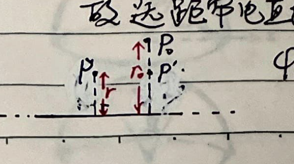
1) On the perpendicular bisector:

$$ E = 2E^+ \cos\theta = 2 \frac{kq}{r^2 + (\frac{l}{2})^2} \frac{\frac{l}{2}}{\sqrt{r^2 + (\frac{l}{2})^2}} = \frac{kql}{\left(r^2 + \frac{l^2}{4}\right)^{\frac{3}{2}}} $$

When $r \gg l$, we have $r_{\pm} \approx r$.

$$ \therefore E \approx \frac{kql}{r^3} = \frac{kp}{r^3} $$

2) On the line connecting the charges:

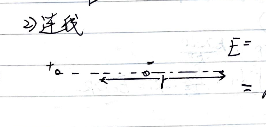$$ E = \frac{kq}{(r - \frac{l}{2})^2} - \frac{kq}{(r + \frac{l}{2})^2} = kq \frac{r^2 + rl + \frac{l^2}{4} - r^2 + rl - \frac{l^2}{4}}{\left[r^2 - (\frac{l}{2})^2\right]^2} \approx kq \cdot \frac{2rl}{r^4} = \frac{2kql}{r^3} $$ $$ \therefore E \approx \frac{2kp}{r^3} $$

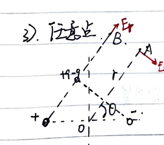
3) Arbitrary point:

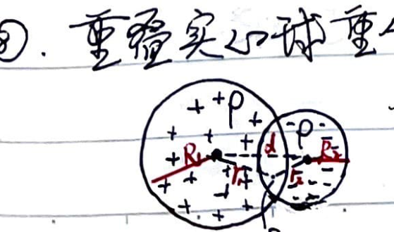
With OA as the polar axis, from $-q$ construct symmetric charge $+q$, and at the same point add $-q$. This decomposes it into two dipoles.

$$ \therefore E_\theta \approx \frac{k q l \sin\theta}{r^3}, \quad E_r \approx \frac{2kq l \cos\theta}{r^3} $$ $$ \therefore E = \sqrt{E_\theta^2 + E_r^2} = \frac{k q l}{r^3} \sqrt{\sin^2\theta + 4\cos^2\theta} = \frac{kp}{r^3} \sqrt{1 + 3\cos^2\theta} $$

⑧ Electric field in the overlapping region of overlapping solid spheres (Volume density $\rho$ and $-\rho$):

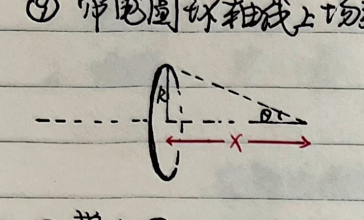
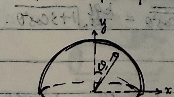
In the overlapping region, for the positive and negative charges at $+P$ and $-P$, we have:

$$ \vec{E}_P = \frac{k \frac{4}{3}\pi r_1^3 \rho}{r_1^3} \vec{r}_1 - \frac{k \frac{4}{3}\pi r_2^3 \rho}{r_2^3} \vec{r}_2 = k \frac{4}{3}\pi \rho (\vec{r}_1 - \vec{r}_2) = \frac{\rho \vec{d}}{3\varepsilon_0} $$

⑨ Electric field distribution on the axis of a charged ring:

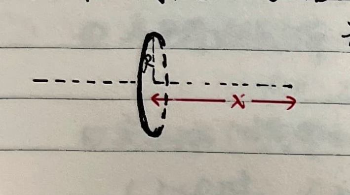
$$ E = \int \frac{k dq}{x^2 + R^2} \cos\theta = \frac{kq}{x^2 + R^2} \frac{x}{\sqrt{x^2 + R^2}} = \frac{qx}{4\pi\varepsilon_0(x^2 + R^2)^{\frac{3}{2}}} $$

⑩ Electric field distribution on the axis of a charged disk:

Using the above result:

$$ E = \int_0^R \frac{(2\pi r dr \sigma) x}{4\pi\varepsilon_0 (x^2 + r^2)^{\frac{3}{2}}} = \frac{\sigma x}{2\varepsilon_0} \int_0^R \frac{r dr}{(x^2 + r^2)^{\frac{3}{2}}} $$ $$ = \frac{\sigma x}{4\varepsilon_0} \int \frac{d(x^2 + r^2)}{(x^2 + r^2)^{\frac{3}{2}}} = \frac{\sigma}{2\varepsilon_0} \left(1 - \frac{x}{\sqrt{x^2 + R^2}}\right) $$

Special Topic: Equivalent Methods for Finding Electric Field Strength

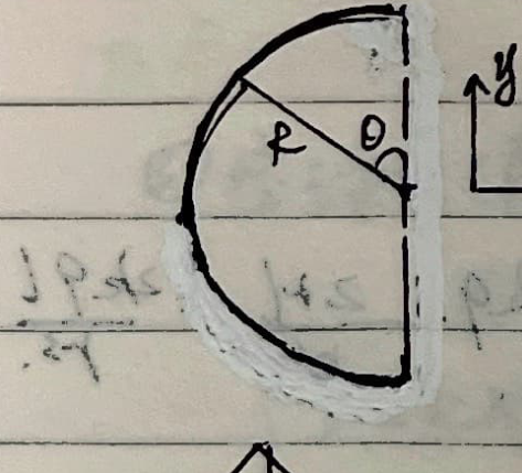
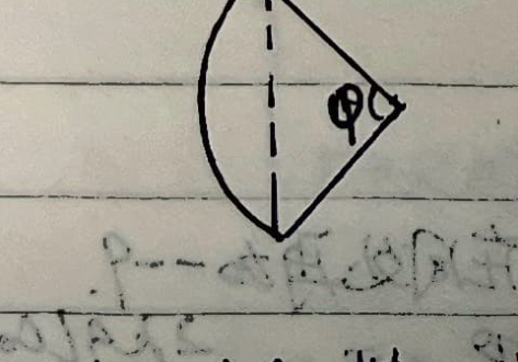
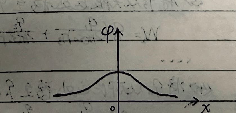
1. Generalizing from the electric field at the center of a uniformly charged semi-circle to an arc with subtended angle $\varphi$:

$$ \begin{cases} dE_y = 0 \quad (\text{by symmetry}) \\ dE_x = \frac{k(\lambda R d\theta)}{R^2} \cos\theta = \frac{k\lambda dy}{R^2} \end{cases} $$ $$ \therefore E = \int dE_x = \frac{k\lambda}{R^2} \int_{-R}^{R} dy = \frac{k\lambda}{R^2} \cdot 2R = E_0 \cdot 2R $$

For an arc with subtended angle $\varphi$:

$$ E = \frac{k\lambda}{R^2} \int dy = \frac{k\lambda}{R^2} \cdot \left(2R \sin\frac{\varphi}{2}\right) $$

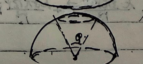
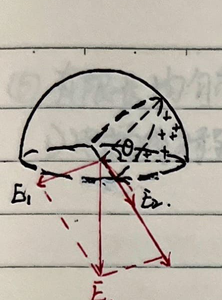
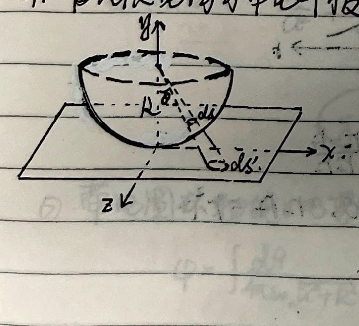
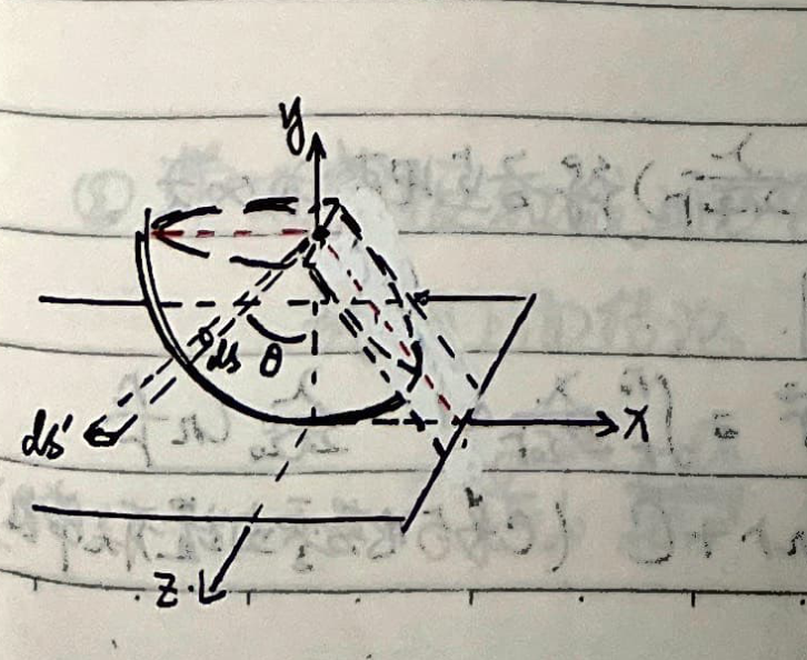
2. Generalizing from the electric field at the center of a uniformly charged hemispherical shell to a spherical cap with subtended angle $\varphi$:

$$ \begin{cases} dE_x = 0 \quad (\text{by symmetry}) \\ dE_y = \frac{k \cdot \sigma dS \cos\theta}{R^2} = \frac{k\sigma dS_x}{R^2} \end{cases} $$ $$ \therefore E = \int dE_y = \frac{k\sigma}{R^2} \int dS_x = \frac{k\sigma}{R^2} \cdot \pi R^2 = E_0 \cdot \pi R^2 $$

For a spherical cap with subtended angle $\varphi$:

$$ E = \frac{k\sigma}{R^2} \int dS_x = \frac{k\sigma}{R^2} \cdot \pi \left(R\sin\frac{\varphi}{2}\right)^2 $$

Alternatively (using $\theta$ for the subtended angle):

$$ \begin{cases} E_1 \cos\frac{\theta}{2} = E_2 \cos\frac{\pi-\theta}{2} \\ E_1 \sin\frac{\theta}{2} + E_2 \sin\frac{\pi-\theta}{2} = E_0 \cdot \pi R^2 \end{cases} $$

Solving yields:

$$ E = (E_0 \cdot \pi R^2) \sin^2\frac{\theta}{2} = \frac{k\sigma}{R^2}(\pi R^2) \sin^2\frac{\theta}{2} $$

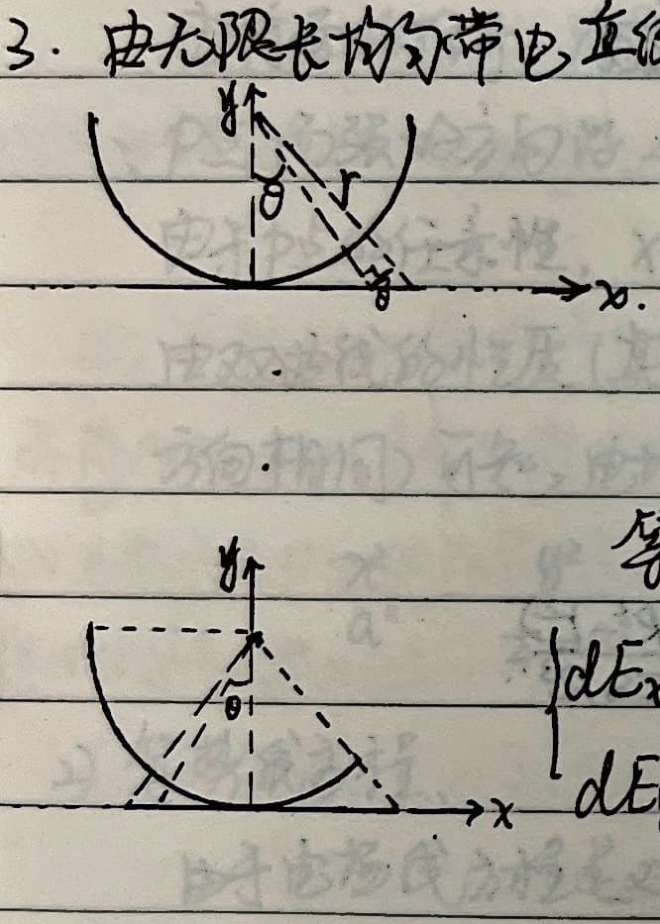
3. Generalizing from the electric field at distance R from an infinitely long uniformly charged line to a finite line:

$$ \begin{cases} dE_x = 0 \quad (\text{by symmetry}) \\ dE_y = \frac{k\lambda dl}{r^2} \cos\theta = \frac{k\lambda (\frac{R}{\cos^2\theta} d\theta)}{(\frac{R}{\cos\theta})^2} \cos\theta = \frac{k\lambda}{R} \cos\theta d\theta \end{cases} $$

This evaluates to $\frac{k(\lambda R d\theta)}{R^2} \cos\theta$, which is equivalent to the electric field at the center of a semi-circle:

$$ \begin{cases} dE_x = \frac{k\lambda dl}{r^2} \sin\theta = \frac{k(\lambda R d\theta)}{R^2} \sin\theta \\ dE_y = \frac{k\lambda dl}{r^2} \cos\theta = \frac{k(\lambda R d\theta)}{R^2} \cos\theta \end{cases} $$

4. Generalizing from the electric field at distance R from an infinitely wide uniformly charged plate to a finite plate:

$$ \begin{cases} dE_x = dE_z = 0 \quad (\text{by symmetry}) \\ dE_y = \frac{k \sigma dS' \cos\theta}{r^2} \end{cases} $$ $$ \because \frac{dS' \cos\theta}{(R/\cos\theta)^2} = \frac{dS}{R^2} \implies dS' = \frac{dS}{\cos^3\theta} $$ $$ \therefore dE_y = \frac{k\sigma \frac{dS}{\cos^3\theta}}{(R/\cos\theta)^2} \cos\theta = \frac{k\sigma dS}{R^2} \quad (\text{Similar to the line segment projection}) $$ $$ \therefore E = \int dE_y = \frac{k\sigma}{R^2} \cdot 2\pi R^2 = 2\pi k \sigma = \frac{\sigma}{2\varepsilon_0} $$

$$ \begin{cases} dE_x = \frac{k\sigma dS'}{r^2} \sin\theta \cos\alpha = \frac{k\sigma dS}{R^2} \tan\theta \cos\alpha \\ dE_y = \frac{k\sigma dS'}{r^2} \cos\theta = \frac{k\sigma dS}{R^2} \\ dE_z = 0 \end{cases} $$

3. Electric Potential

$$ \varphi_A = \int_A^\infty \vec{E} \cdot d\vec{l} $$ $$ \begin{cases} \varphi_A = \frac{1}{4\pi\varepsilon_0} \sum \frac{q_i}{r_i} \quad (\text{discrete}) \\ \varphi_A = \frac{1}{4\pi\varepsilon_0} \int \frac{dq}{r} \quad (\text{continuous}) \end{cases} $$

When infinity is non-conducting, potential at infinity is zero. If not considering the charge of the Earth, Earth is regarded as potential zero.

① Electric potential distribution of a point charge:

$$ \varphi_a = \frac{q}{4\pi\varepsilon_0} \int_a^\infty \frac{dr}{r^2} = \frac{q}{4\pi\varepsilon_0} \left(-\frac{1}{r}\right)_a^\infty = \frac{q}{4\pi\varepsilon_0 a} $$ $$ U_{ab} = \varphi_a - \varphi_b = \frac{q}{4\pi\varepsilon_0}\left(\frac{1}{a} - \frac{1}{b}\right) $$

② Solid sphere:

$$ \begin{cases} r \ge R, \quad \varphi = \int_r^\infty E dr = \frac{q}{4\pi\varepsilon_0 r} \\ r < R, \quad \varphi = \frac{q}{4\pi\varepsilon_0 R} + \int_r^R \frac{q \cdot r dr}{4\pi\varepsilon_0 R^3} = \frac{q}{4\pi\varepsilon_0 R} + \frac{q(R^2 - r^2)}{8\pi\varepsilon_0 R^3} = \frac{q(3R^2 - r^2)}{8\pi\varepsilon_0 R^3} \end{cases} $$

③ Hollow spherical shell:

$$ \begin{cases} r \ge R, \quad \varphi = \frac{q}{4\pi\varepsilon_0 r} \\ r < R, \quad \varphi = \frac{q}{4\pi\varepsilon_0 R} \end{cases} $$

④ Electric Dipole:

$$ \varphi = \frac{q}{4\pi\varepsilon_0 r_+} - \frac{q}{4\pi\varepsilon_0 r_-} = \frac{q}{4\pi\varepsilon_0} \frac{r_- - r_+}{r_- r_+} $$

When $r \gg l$, we have $r_- - r_+ \approx l \cos\theta$, $r_- r_+ \approx r^2$.

$$ \therefore \varphi \approx \frac{q}{4\pi\varepsilon_0} \frac{l \cos\theta}{r^2} = \frac{\vec{p} \cdot \vec{r}}{4\pi\varepsilon_0 r^3} $$

⑤ Electric potential distribution of infinitely long uniformly charged line:

If we still choose infinity as the zero potential point, then from $\int_r^\infty E dr$ ($E = \frac{\lambda}{2\pi\varepsilon_0 r}$) we get the potential at each point is infinity. So we choose a point $P_0$ at distance $r_0$ from the charged line as the zero potential point. As shown in the figure:

$$ \varphi_P = \int_P^{P_0} \vec{E} \cdot d\vec{r} = \int_r^{r_0} \frac{\lambda}{2\pi\varepsilon_0 r} dr = \frac{\lambda}{2\pi\varepsilon_0} \ln\frac{r_0}{r} $$ $$ = -\frac{\lambda}{2\pi\varepsilon_0} \ln r + \frac{\lambda}{2\pi\varepsilon_0} \ln r_0 = -\frac{\lambda}{2\pi\varepsilon_0} \ln r + C \quad (C \text{ is a constant related to the zero potential point}) $$

⑥ Electric field lines and equipotential lines equations for a finite length uniformly charged straight line:

1) Electric field line equation:

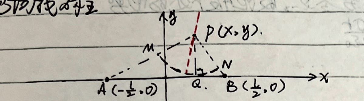
From the previous derivation, the effect of AB on P is equivalent to that of arc MN (with the same linear density $\lambda$) on P. $\therefore$ The direction of the electric field at point P is along the angle bisector of $\angle MPN$, which is also the tangent direction of the electric field line.

Due to the arbitrariness of point P, the direction of the electric field at any point on the $xy$ plane is along the bisector of $\angle APB$.

From the properties of a hyperbola (the tangent direction at any point on it is the same as the angle bisector of the lines connecting the two foci to that point), it can be known that the electric field lines are a family of confocal hyperbolas. Their equation is:

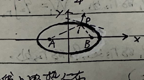
$$ \frac{x^2}{a^2} - \frac{y^2}{\frac{l^2}{4} - a^2} = 1 \quad \left(\text{where } 0 < a < \frac{l}{2}\right) $$

2) Equipotential line equation:

Since the electric field line equation is a hyperbola, and equipotential lines are everywhere perpendicular to the electric field lines, the equipotential line equation is an ellipse:

$$ \frac{x^2}{a^2} + \frac{y^2}{a^2 - \frac{l^2}{4}} = 1 \quad \left(\text{where } a > \frac{l}{2}\right) $$

⑦ Electric potential distribution on the axis of a charged ring:

$$ \varphi = \int \frac{dq}{4\pi\varepsilon_0\sqrt{x^2+R^2}} = \frac{q}{4\pi\varepsilon_0\sqrt{x^2+R^2}} $$

⑧ Electric potential distribution on the axis of a charged disk:

Using the above result:

$$ \varphi = \int \frac{dq}{4\pi\varepsilon_0\sqrt{x^2+r^2}} = \int_0^R \frac{2\pi r dr \sigma}{4\pi\varepsilon_0\sqrt{x^2+r^2}} $$ $$ = \frac{\sigma}{2\varepsilon_0} \int_0^R \frac{r dr}{\sqrt{x^2+r^2}} = \frac{\sigma}{4\varepsilon_0} \int_0^R \frac{d(x^2+r^2)}{\sqrt{x^2+r^2}} = \frac{\sigma}{2\varepsilon_0}\left(\sqrt{x^2+R^2} - x\right) $$

⑨ Electric potential distribution of an infinitely wide uniformly charged flat plate:

Choosing the charged plane itself as the zero potential point, the potential at a distance $r$ from the plate is:

$$ \varphi = -\int_0^r \frac{\sigma}{2\varepsilon_0} dr = -\frac{\sigma r}{2\varepsilon_0} $$

4. Electric Potential Energy and Electrostatic Energy

① Electric Potential Energy:

Because the electrostatic field is a conservative field, when moving a charge in an electrostatic field, the work done by the electrostatic field force is independent of the path. Therefore, any charge in an electrostatic field has electrostatic potential energy.

$$ W = q\varphi $$ $$ A_{12} = W_1 - W_2 = q(\varphi_1 - \varphi_2) $$

The electric potential energy of a charge in an external electric field is shared by the charge and the charge system that produces the electric field. It is an interaction energy. Similarly, the electric potential energy of a point charge system in an external electric field is $W = \sum q_i \varphi_i$.

(Note: $\varphi_i$ does not include the potential produced by the charges within this charge system at that point.)

② Electrostatic Energy:

1) Mutual energy: The work done by electrostatic forces between charges when they are scattered from their current positions to infinity. i.e., the interaction energy of a point charge system.

Moving $q_1$ from infinity to a point in space, no work is done.
Moving $q_2$ from infinity to distance $r_{12}$ from $q_1$: $W_1 = q_2 \int_{r_{12}}^\infty \frac{q_1 dr}{4\pi\varepsilon_0 r^2} = \frac{q_1 q_2}{4\pi\varepsilon_0 r_{12}}$.
Moving $q_3$ from infinity to distance $r_{13}$ from $q_1$ and $r_{23}$ from $q_2$: $W_2 = q_3 \left(\frac{q_1}{4\pi\varepsilon_0 r_{13}} + \frac{q_2}{4\pi\varepsilon_0 r_{23}}\right)$.
$\dots$
Moving $q_n$ from infinity to distance $r_{1n}$ from $q_1$ $\dots$ $r_{(n-1)n}$ from $q_{n-1}$: $W_n = q_n \left(\frac{q_1}{4\pi\varepsilon_0 r_{1n}} + \frac{q_2}{4\pi\varepsilon_0 r_{2n}} + \dots + \frac{q_{n-1}}{4\pi\varepsilon_0 r_{(n-1)n}}\right)$.

$$ \therefore E = \sum_{i=1}^n W_i = \frac{1}{2} \sum_{i=1}^n q_i \varphi_i $$

2) Self-energy: The work done by electrostatic forces when a charged body is divided into infinite charge elements and scattered to infinity from each other.

$$ E = \frac{1}{2} \int \varphi dq $$

Therefore, the total electrostatic energy in space = mutual energy + self-energy = $\frac{1}{2} \int \varphi dq$.

$$ = \int w dV = \frac{1}{2} \varepsilon_0 \int E^2 dV \quad (w: \text{energy density}) $$

③ Applications of Energy

1) Electric potential energy of an electric dipole in an external uniform electric field $\vec{E}$:

$$ W = \sum_{i=1}^n q_i \varphi_i = q\varphi_A + (-q\varphi_B) $$ $$ = -q E l \cos\theta = -\vec{p} \cdot \vec{E} $$

2) Electrostatic energy of a parallel plate capacitor:

$$ \begin{cases} W = \frac{1}{2} \int \varphi dq = \frac{1}{2} q(U_1 - U_2) = \frac{1}{2} qU \\ W = \frac{1}{2}\varepsilon_0 \int E^2 dV = \frac{1}{2}\varepsilon_0 E^2 S \cdot d = \frac{1}{2}\varepsilon_0 \frac{U^2}{d^2} S \cdot d = \frac{1}{2} C U^2 \\ W = \int q dU = \int \frac{q dq}{C} = \frac{1}{2} \frac{q^2}{C} \end{cases} $$

3) Solid sphere:

$$ \begin{cases} \text{When } r < R, \quad W = \frac{1}{2} \varepsilon_0 \int_0^R \left(\frac{qr}{4\pi\varepsilon_0 R^3}\right)^2 4\pi r^2 dr = \frac{1}{2}\varepsilon_0 \left(\frac{q}{4\pi\varepsilon_0 R^3}\right)^2 4\pi \int_0^R r^4 dr = \frac{q^2}{40\pi\varepsilon_0 R} \\ \text{When } r \ge R, \quad W = \frac{1}{2} \varepsilon_0 \int_R^\infty \left(\frac{q}{4\pi\varepsilon_0 r^2}\right)^2 4\pi r^2 dr = \frac{1}{2}\varepsilon_0 \left(\frac{q}{4\pi\varepsilon_0}\right)^2 4\pi \int_R^\infty \frac{dr}{r^2} = \frac{q^2}{8\pi\varepsilon_0 R} \end{cases} $$ $$ \therefore W_{\text{total}} = \frac{q^2}{40\pi\varepsilon_0 R} + \frac{q^2}{8\pi\varepsilon_0 R} = \frac{3q^2}{20\pi\varepsilon_0 R} $$

Alternatively using $W = \frac{1}{2} \int \varphi dq$:

$$ W_{\text{total}} = \frac{1}{2} \int \varphi dq = \frac{1}{2} \int_0^R \frac{q(3R^2-r^2)}{8\pi\varepsilon_0 R^3} \cdot \frac{q}{\frac{4}{3}\pi R^3} 4\pi r^2 dr = \frac{3q^2}{20\pi\varepsilon_0 R} $$

4) Hollow spherical shell:

$$ \begin{cases} \text{When } r < R, \quad W = 0 \\ \text{When } r \ge R, \quad W = \frac{1}{2} \varepsilon_0 \int_R^\infty \left(\frac{q}{4\pi\varepsilon_0 r^2}\right)^2 4\pi r^2 dr = \frac{q^2}{8\pi\varepsilon_0 R} \end{cases} $$ $$ \therefore W_{\text{total}} = \frac{q^2}{8\pi\varepsilon_0 R} $$

Alternatively:

$$ W_{\text{total}} = \frac{1}{2} \int \varphi dq = \frac{1}{2} \cdot \frac{q}{4\pi\varepsilon_0 R} \cdot q = \frac{q^2}{8\pi\varepsilon_0 R} $$

5. Conductors and Dielectrics

① Conductors in electrostatic equilibrium:

$$ \begin{cases} \text{Inside: } \vec{E} = \vec{E}_{\text{external}} + \vec{E}_{\text{induced}} = 0 \\ \text{Outside: } \text{Field strength at outer surface } \vec{E} = \frac{\sigma}{\varepsilon_0} \vec{n} \perp \text{outer surface} \end{cases} $$

The conductor is an equipotential body, its surface is an equipotential surface, and induced charges distribute on the surface.

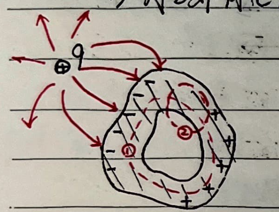
Conductor with a cavity:

1) Charges outside cavity, conductor ungrounded, no charge on inner wall, no electric field inside cavity.

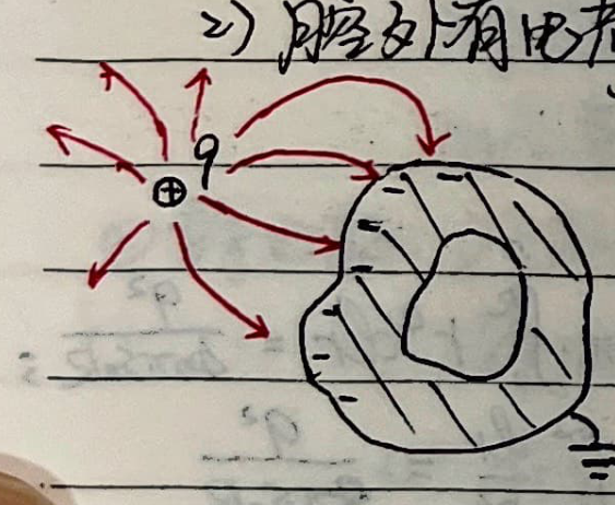
Proof: Take a Gaussian surface $S$ inside the conductor enclosing the cavity. Since $\Phi = \oint_S \vec{E} \cdot d\vec{S} = 0$, the net charge on the inner wall is zero. Take a loop $L$, according to the circuital law, there are no electric field lines inside the cavity, so there is no charge on the inner wall. Hence, no electric field inside.

2) Charges outside cavity, conductor grounded, no charge on inner wall, only one type of charge on outer surface, no electric field inside cavity.

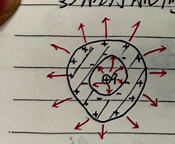
Proof: If positive charges exist on the outer surface (as shown), the electric field lines they emit will extend to infinity (they cannot end at negative charges on the other side of the conductor because the potential is equal everywhere). But the potential at infinity is also zero, which contradicts the existence of electric field lines connecting the conductor and infinity.

3) Charge inside cavity, conductor ungrounded, inner and outer wall charges are $-q$ and $+q$ respectively, electric field exists outside cavity.

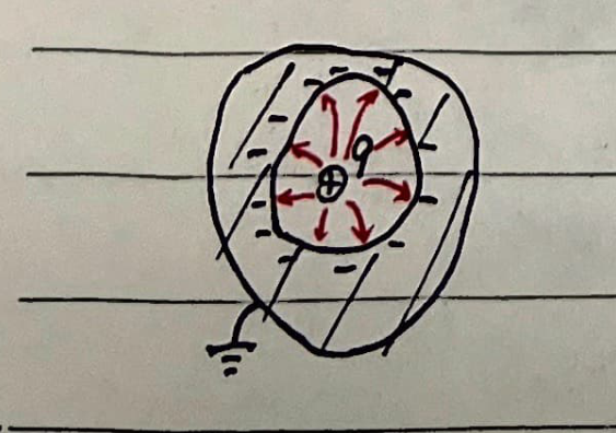
Proof: Take a Gaussian surface inside the conductor enclosing the cavity. Since $\oint_S \vec{E} \cdot d\vec{S} = 0$, the charge on the inner wall is $-q$ to cancel the charge $+q$ in the cavity. Take a Gaussian surface outside enclosing the conductor, due to charge conservation, the outer surface has $+q$, so the net charge is $+q$, $\oint_S \vec{E} \cdot d\vec{S} \neq 0$, thus there is an electric field outside.

4) Charge inside cavity, conductor grounded, inner wall charge $-q$, outer wall charge $0$, no electric field outside cavity.

Proof: Take a Gaussian surface inside the conductor enclosing the cavity. Since $\oint_S \vec{E} \cdot d\vec{S} = 0$, the inner wall has $-q$. Also, since the potential inside the conductor (including the outer surface) is zero, and the potential at infinity is zero, there is no electric field outside.

In summary: Cases 1) and 2): outside does not affect inside. Case 3): inside does not affect outside. If charges exist both inside and outside simultaneously (grounded or ungrounded), then superpose the respective cases.

② Dielectrics in electrostatic equilibrium:

$$ \begin{cases} \text{Polar molecules } \to \text{inherent electric moment } \to \text{inherent moments align in external field} \\ \text{Non-polar molecules } \to \text{induced electric moment } \to \text{external field separates centers of positive and negative charges} \end{cases} $$

Macroscopic effect: generates surface polarization charges.

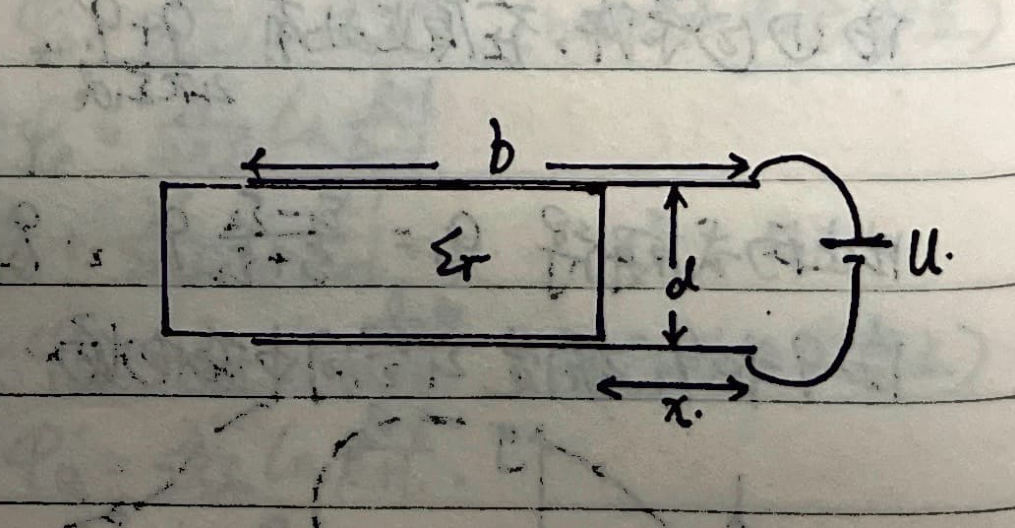
Let the external field be $\vec{E}_0$. The surface density of polarization charges is $\sigma'$. The field induced by it is $\vec{E}'$. The relative permittivity of the dielectric is $\varepsilon_r$. Therefore, the resultant field in space is $\vec{E} = \vec{E}_0 + \vec{E}'$.

Take a rectangular cuboid dielectric as an example:

From the generalized Gauss's law: $\varepsilon_0 \oint_S (\varepsilon_r \vec{E}) \cdot d\vec{S} = q_{\text{free charges}}$

Take a Gaussian surface as shown in the diagram: $\because q_{\text{free}} = 0 \quad \therefore -\varepsilon_0 E_0 + \varepsilon_0 \varepsilon_r (E_0 - E') = 0 \quad \therefore E' = \frac{\varepsilon_r - 1}{\varepsilon_r} E_0$.

$$ \therefore \text{Resultant field inside dielectric } E = E_0 - E' = \frac{E_0}{\varepsilon_r} $$

Again by Gauss's law: $\varepsilon_0(-E_0 \Delta S + E \Delta S) = -\sigma' \Delta S$. Solving yields: $-\sigma' = -\frac{\varepsilon_0(\varepsilon_r-1)}{\varepsilon_r} E_0$.

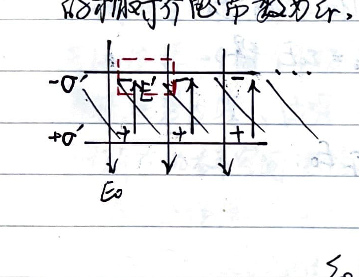
In summary: From initial conditions $E_0$ and $\varepsilon_r$, by Gauss's law:

$$ \begin{cases} \varepsilon_0 \oint_S \vec{E} \cdot d\vec{S} = q_{\text{free}} + q_{\text{polarization}} \\ \varepsilon_0 \oint_S (\varepsilon_r \vec{E}) \cdot d\vec{S} = q_{\text{free}} \end{cases} $$

(Note: A dielectric is generally not an equipotential body, its surface is generally not an equipotential surface, and polarization charges distribute on the surface.)

We can solve for:

$$ E = \frac{E_0}{\varepsilon_r}, \quad E' = \frac{\varepsilon_r-1}{\varepsilon_r} E_0, \quad \sigma' = \frac{\varepsilon_0(\varepsilon_r-1)}{\varepsilon_r} E_0 $$

Define polarization $\vec{P} = \varepsilon_0(\varepsilon_r-1)\vec{E}$, then $\sigma' = \frac{\vec{P} \cdot d\vec{S}}{dS} = \vec{P} \cdot \hat{n}$.

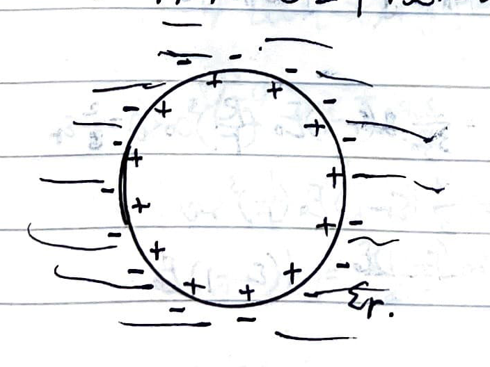
1) Sphere of radius R, charge q immersed in a dielectric $\varepsilon_r$:

From $\varepsilon_0 \oint (\varepsilon_r \vec{E}) \cdot d\vec{S} = q$, we get $\varepsilon_0 \varepsilon_r E \cdot 4\pi r^2 = q \quad \therefore E = \frac{q}{4\pi\varepsilon_0\varepsilon_r r^2}$.

From $\varepsilon_0 \oint \vec{E} \cdot d\vec{S} = q + q'$, we get $q' = \varepsilon_0 \cdot \frac{q}{4\pi\varepsilon_0\varepsilon_r r^2} \cdot 4\pi r^2 - q = \frac{q}{\varepsilon_r} - q = -\frac{\varepsilon_r-1}{\varepsilon_r} q$.

2) Half space between two parallel metal plates ($+\sigma_0, -\sigma_0$) is filled with dielectric $\varepsilon_r$. (See next page)

2) Half space between two parallel metal plates ($+\sigma_0, -\sigma_0$) is filled with dielectric $\varepsilon_r$.

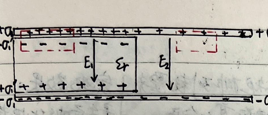
From charge conservation: $\sigma_1 + \sigma_2 = 2\sigma_0$.

From Gauss's law:

In the dielectric: $(\sigma_1 \Delta S - \sigma_1' \Delta S) = \varepsilon_0 E_1 \Delta S \quad \therefore \sigma_1 - \sigma_1' = \varepsilon_0 E_1$.
Alternatively: $\sigma_1 \Delta S = \varepsilon_0 \varepsilon_r E_1 \Delta S \quad \therefore \sigma_1 = \varepsilon_0 \varepsilon_r E_1$.
In the vacuum: $\sigma_2 \Delta S = \varepsilon_0 E_2 \Delta S \quad \therefore \sigma_2 = \varepsilon_0 E_2$.

Also $\because U_1 = U_2 \quad \therefore E_1 = E_2$.

Thus from the equations we get:

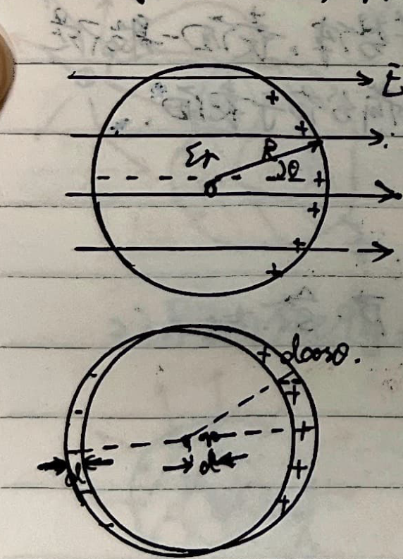
$$ \begin{cases} \sigma_1 = \frac{2\varepsilon_r}{1+\varepsilon_r} \sigma_0 \\ \sigma_2 = \frac{2}{1+\varepsilon_r} \sigma_0 \\ \sigma_1' = \frac{2(\varepsilon_r-1)}{1+\varepsilon_r} \sigma_0 \end{cases} \quad \text{and} \quad E_1 = E_2 = \frac{2\sigma_0}{\varepsilon_0(1+\varepsilon_r)} = \frac{2}{1+\varepsilon_r} E_0 $$

3) Dielectric sphere of radius R, relative permittivity $\varepsilon_r$ in a uniform field $E_0$:

At polar angle $\theta$, the polarization is $\vec{P} = \varepsilon_0(\varepsilon_r - 1)\vec{E}_0$ (using external field as approximation).

$$ \sigma' = \vec{P} \cdot \hat{n} = P \cos\theta = \varepsilon_0(\varepsilon_r - 1)E_0 \cos\theta $$

This surface charge distribution is equivalent to two spheres with volume charge density $\rho$ and $-\rho$ separated by distance $d$ (where $d \ll R$).

The total positive polarization charge on the right hemisphere is:

$$ q_{\text{polar}}' = \int_0^{\pi/2} \sigma' \cdot 2\pi R\sin\theta \cdot R d\theta = \varepsilon_0(\varepsilon_r - 1)E_0 \pi R^2 $$

The polarized sphere is equivalent to an electric dipole with moment $p' = P \cdot \frac{4}{3}\pi R^3$.

Therefore, the electric field outside the sphere is:

$$ \begin{cases} E_r = \frac{1}{4\pi\varepsilon_0} \frac{2p'\cos\theta}{r^3} = \frac{2}{3}(\varepsilon_r - 1)E_0 \left(\frac{R}{r}\right)^3 \cos\theta \\ E_\theta = \frac{1}{4\pi\varepsilon_0} \frac{p'\sin\theta}{r^3} = \frac{1}{3}(\varepsilon_r - 1)E_0 \left(\frac{R}{r}\right)^3 \sin\theta \end{cases} $$

The induced electric field inside the sphere is $E' = \frac{1}{3}(\varepsilon_r - 1)E_0$.

Special Topic: Method of Images

Principle: Replace the effect of induced charges with one or several point charges.
Essence: In the space where the original charges are located, the spatial electric field strength and potential distribution remain unchanged.
Reason: Uniqueness Theorem.

1. Infinite grounded flat plate:

Since the plate is grounded, its potential is 0. The potential on the perpendicular bisector plane of an electric dipole is also 0. We can imagine a negative charge $-q$ at the mirror image point of $+q$ with respect to the plate to ensure the plate's potential is zero. By the Uniqueness Theorem, replacing the grounded plate with $-q$ leaves the electric field in the right half-space unchanged.

Field distribution on the plate is $E = \frac{k \cdot 2q a}{(r^2 + a^2)^{3/2}}$, with direction perpendicular to the plate.

$$ \therefore \sigma = \varepsilon_0 E = -\frac{q a}{2\pi (r^2 + a^2)^{3/2}} $$

Total charge on the plate $q' = \int_0^\infty \sigma \cdot 2\pi r dr = -q$. Therefore, there is no electric field in the left space of the plate, and $+q$ experiences an electrostatic force from the induced charges on the plate $F = \frac{k q^2}{(2a)^2}$, equivalent to the force from the image charge $-q$.

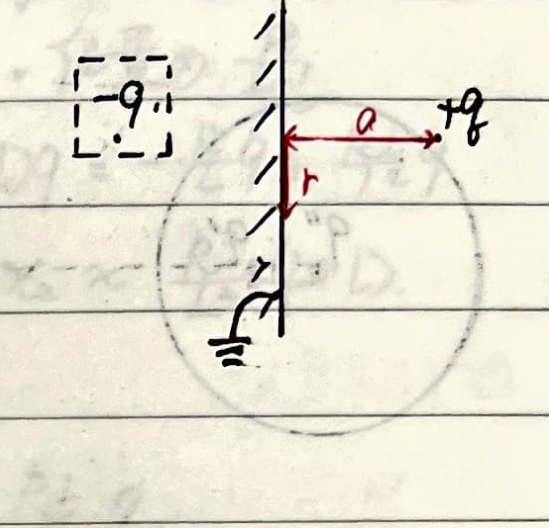
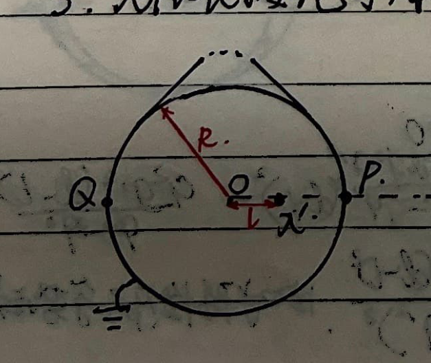
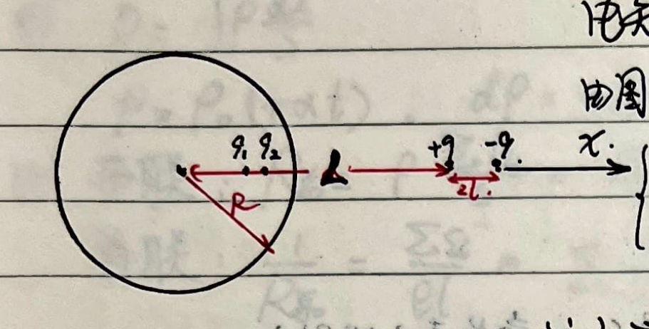
2. Grounded conducting spherical shell:

Suppose a positive charge $q$ and a negative charge $q'$ ($|q'| < q$) exist in space. The equipotential surface $\varphi = 0$ is a spherical surface.

Proof: $\because U_0 = 0 \implies \frac{kq'}{\sqrt{x^2+y^2}} + \frac{kq}{\sqrt{(d-x)^2+y^2}} = 0$. Squaring and rearranging:

$$ q^2 (x^2+y^2) = q'^2 [(d-x)^2+y^2] \implies q^2 x^2 + q^2 y^2 = q'^2(d^2 - 2dx + x^2) + q'^2 y^2 $$

Completing the square yields:

$$ \left( x + \frac{q'^2 d}{q^2 - q'^2} \right)^2 + y^2 = \frac{q^2 q'^2 d^2}{(q^2 - q'^2)^2} $$

From symmetry, the equipotential surface is a sphere. From this, for a point charge $q$ at distance $d$ from the center of a conducting sphere of radius $R$, the field outside can be evaluated by an image charge $q'$ inside.

The image charge $q'$ is at a distance $l = \frac{q'^2 d}{q^2 - q'^2}$ from the center, and the sphere radius is $R = \frac{q q' d}{q^2 - q'^2}$. Solving gives:

$$ q' = -\frac{R}{d} q, \quad l = \frac{R^2}{d} $$

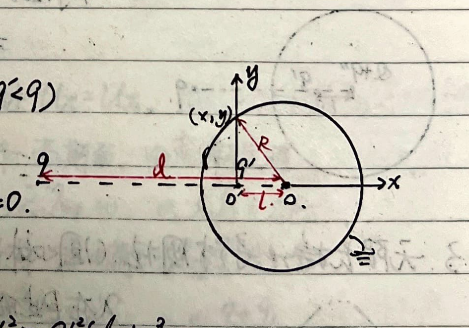
Also, since the potential at the center $O$ is $0$ in a grounded shell, $\frac{k q'}{l} + \frac{k q_{\text{induced}}}{R} = 0$, thus the total induced charge on the spherical surface equals the image charge $q'$.

Discussion:

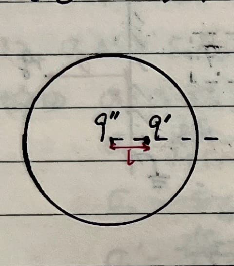
① If initially the spherical shell is ungrounded and uncharged, and $+q$ is placed outside:

1) To ensure the sphere is an equipotential body, place $q' = -\frac{R}{d} q$ at $l = \frac{R^2}{d}$ to make the shell potential zero.

2) Because $+q$ was added, the shell's net charge must remain zero. To ensure the shell is equipotential and the net charge is zero, a layer $q'' = -q' = \frac{R}{d} q$ should be uniformly distributed on the surface. And $q''$ uniformly distributed on the surface is equivalent to a point charge at the center.

In summary: image charges are $q' = -\frac{R}{d} q$ at $x = \frac{R^2}{d}$, and $q'' = \frac{R}{d} q$ at $x = 0$.

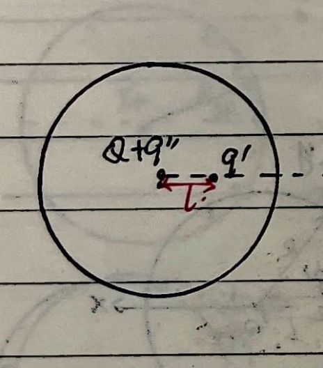
② If initially the shell is ungrounded and carries charge $Q$, and $+q$ is added outside:

Similarly, add $q' = -\frac{R}{d} q$ at $l = \frac{R^2}{d}$ to make $\varphi = 0$.

Add $q'' = \frac{R}{d} q$ at the center to make net charge zero ($\varphi = \frac{k q''}{R} = \frac{k q}{d}$).

Add $q''' = Q$ at the center to make the net charge $Q$. The final potential is $\varphi = \frac{k(Q + \frac{R}{d}q)}{R}$.

3. Infinitely long grounded conducting cylinder (with line charge $\lambda$ at distance $d$ outside):

The potential from $\lambda$ at point $P$ is $\varphi_P = \frac{\lambda}{2\pi\varepsilon_0} \ln\frac{r_0}{d-R}$.

The potential from image line $\lambda'$ at $P$ is $\varphi_P' = \frac{\lambda'}{2\pi\varepsilon_0} \ln\frac{r_0}{R-l}$.

Since the cylinder is grounded, the potential at $P$ and $Q$ must be zero:

$$ \begin{cases} \frac{\lambda}{2\pi\varepsilon_0} \ln\frac{r_0}{d-R} + \frac{\lambda'}{2\pi\varepsilon_0} \ln\frac{r_0}{R-l} = 0 \\ \frac{\lambda}{2\pi\varepsilon_0} \ln\frac{r_0}{d+R} + \frac{\lambda'}{2\pi\varepsilon_0} \ln\frac{r_0}{R+l} = 0 \end{cases} $$

Solving these yields: $\lambda' = -\lambda$ and $l = \frac{R^2}{d}$.

4. Electric dipole outside an ungrounded spherical shell at distance $L$:

Dipole moment $P = q \cdot 2l$. Coordinate of $+q$ is $L+l$, coordinate of $-q$ is $L-l$.

Image of $+q$ is $q_1 = -\frac{R}{L+l} q$ at position $x_1 = \frac{R^2}{L+l}$.

Image of $-q$ is $q_2 = +\frac{R}{L-l} q$ at position $x_2 = \frac{R^2}{L-l}$.

Since $L \gg l$:

$$ q_1 \approx -\frac{R}{L}\left(1-\frac{l}{L}\right)q = -\frac{R}{L}q + \frac{Rl}{L^2}q, \quad x_1 \approx \frac{R^2}{L^2}(L-l) $$ $$ q_2 \approx +\frac{R}{L}\left(1+\frac{l}{L}\right)q = \frac{R}{L}q + \frac{Rl}{L^2}q, \quad x_2 \approx \frac{R^2}{L^2}(L+l) $$

The image dipole moment is $p' \approx q_2 \cdot (x_2-x_1) = \frac{R}{L}q \cdot \frac{2R^2 l}{L^2} = \frac{R^3}{L^3} P$.

Additionally, at the midpoint of $q_1, q_2$ (which is $\approx \frac{R^2}{L}$), there is a net image point charge: $q' = q_1 + q_2 = \frac{2Rl}{L^2}q$.

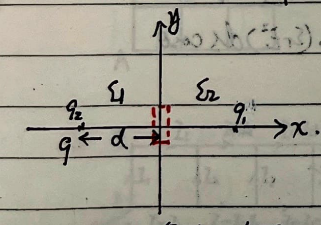
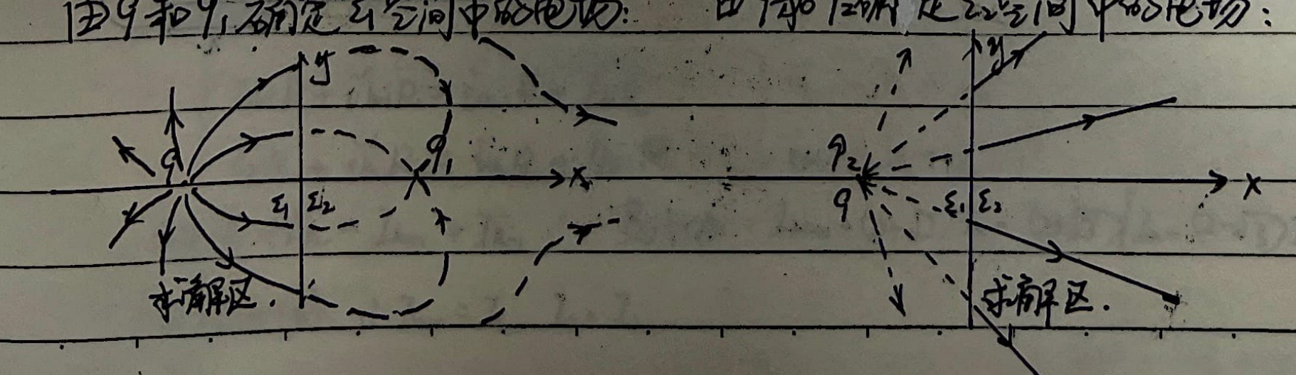
5. Image of a point charge with respect to an infinite dielectric plane:

Conditions:

① At the dielectric interface, $U_{\text{left}} = U_{\text{right}}$.

② Make a Gaussian pillbox near the origin. From Gauss's law $\Sigma \oint (\varepsilon_r \vec{E}) \cdot d\vec{S} = \Sigma q_{\text{free}} = 0 \implies \varepsilon_1 E_1 = \varepsilon_2 E_2$.

Assume there are image charges $q_1, q_2$ at $x = \pm d$ respectively. From conditions ① and ② at the origin:

$$ \begin{cases} \frac{q+q_1}{4\pi\varepsilon_0 d} = \frac{q_2}{4\pi\varepsilon_0 d} \\ \varepsilon_1 \frac{q-q_1}{4\pi\varepsilon_0 d^2} = \varepsilon_2 \frac{q_2}{4\pi\varepsilon_0 d^2} \end{cases} $$

Solving these yields: $q_1 = \frac{\varepsilon_1 - \varepsilon_2}{\varepsilon_1 + \varepsilon_2} q$ and $q_2 = \frac{2\varepsilon_1}{\varepsilon_1 + \varepsilon_2} q$.

$q$ and $q_1$ determine the electric field in the left space; $q_2$ determines the electric field in the right space.

Special Topic: Principle of Virtual Work in Electrostatic Fields

1. Electrostatic force experienced by the plates of a parallel plate capacitor:

① When $q$ is constant:

$$ W = \frac{1}{2}\varepsilon_0 E^2 S d = \frac{1}{2}\varepsilon_0 \left(\frac{q}{\varepsilon_0 S}\right)^2 S d = \frac{1}{2} \frac{q^2 d}{\varepsilon_0 S} $$ $$ \therefore F = -\frac{\partial W}{\partial d} = -\frac{q^2}{2\varepsilon_0 S} = -\frac{\sigma^2 S}{2\varepsilon_0} = -\frac{1}{2}\varepsilon_0 E^2 S $$

The negative sign indicates an attractive force.

② When $U$ is constant:

$$ W = \frac{1}{2}\varepsilon_0 \left(\frac{U}{d}\right)^2 S d = \frac{1}{2} \frac{\varepsilon_0 U^2 S}{d} $$ $$ \therefore F = \frac{\partial W}{\partial d} = -\frac{\varepsilon_0 U^2 S}{2d^2} = -\frac{1}{2}\varepsilon_0 E^2 S $$

The negative sign indicates an attractive force.

In summary, $|F| = \frac{1}{2}\varepsilon_0 E^2 S$, which can be generalized to any charged body. The electrostatic pressure is $f = \frac{dF}{dS} = \frac{1}{2}\varepsilon_0 E^2 = w_e$.

$$ F = \int_S p dS = \frac{1}{2\varepsilon_0} \int_S \sigma^2 dS. \quad \text{Also } W = \int_V \frac{1}{2}\varepsilon_0 E^2 dV $$ $$ F = \int_S \frac{1}{2}\varepsilon_0 (\varepsilon_r E^2) dS \cos\theta $$

2. Interaction force between the upper and lower hemispheres of a charged conducting sphere:

$$ F = \frac{1}{2\varepsilon_0} \int_S \sigma^2 dS \cos\theta = \frac{\sigma^2}{2\varepsilon_0} \pi R^2 $$

3. Force pulling a dielectric block inside parallel metal plates:

$$ W = \frac{1}{2} \left( \frac{\varepsilon_0 \varepsilon_r (b-x) l}{d} + \frac{\varepsilon_0 x l}{d} \right) U^2 $$ $$ \therefore F = \frac{\partial W}{\partial x} = -\frac{\varepsilon_0 (\varepsilon_r - 1) l U^2}{2d} $$

Special Topic: Model of Conductor Reaching Electrostatic Equilibrium

1. Decay of Current Density

Let the surface charge density accumulated on both ends of the conductor at time $t$ be $\sigma_e$. $\sigma_e$ generates an opposing electric field $E'$ inside the conductor, then $E = E_0 - E'$, which is the resultant field inside the conductor.

From Gauss's Law:

$$ -E_0 \Delta S + (E_0 - E') \Delta S = \frac{(-\sigma_e) \Delta S}{\varepsilon_0} $$ $$ \therefore E' = \frac{\sigma_e}{\varepsilon_0} $$

Also, since $dq = i dt \implies d\sigma_e \cdot S = j \cdot S dt = \sigma E \cdot S dt$

$$ \therefore d\sigma_e = \sigma E dt = \sigma\left(E_0 - \frac{\sigma_e}{\varepsilon_0}\right) dt $$ $$ \therefore \int_0^{\sigma_e} \frac{d\sigma_e}{E_0 - \frac{\sigma_e}{\varepsilon_0}} = \int_0^t \sigma dt \implies \sigma_e = \varepsilon_0 E_0 (1 - e^{-\frac{\sigma}{\varepsilon_0} t}) $$

And $E' = E_0 (1 - e^{-\frac{\sigma}{\varepsilon_0} t})$

Therefore, $E = E_0 e^{-\frac{\sigma}{\varepsilon_0} t}$

$$ j = \sigma E = \sigma E_0 e^{-\frac{\sigma}{\varepsilon_0} t} $$

It can be seen that at $t=0$, $j = \sigma E_0$; as $t$ increases, $j$ decays exponentially; when $t \to \infty$, $j=0$, reaching electrostatic equilibrium.

2. Establishing a steady current:

In a conductor element, because $\vec{j} = \sigma \vec{E}$, $\oint \vec{E} \cdot d\vec{S} = \frac{q}{\varepsilon_0}$.

$$ \therefore \frac{1}{\sigma} \oint \vec{j} \cdot d\vec{S} = \frac{1}{\varepsilon_0} q $$

From the continuity equation of current: $\oint \vec{j} \cdot d\vec{S} = -\frac{dq}{dt}$, we get

$$ -\frac{dq}{dt} = \frac{\sigma}{\varepsilon_0} q $$

$\therefore$ The accumulated charge in the conductor element is $q = q_0 e^{-\frac{\sigma}{\varepsilon_0} t}$.