Part 9: Resistance, Capacitance, Inductance

1. Resistance

① Resistivity and Temperature:

$$ R = \rho \frac{l}{S} $$ $$ \rho = \rho_0(1+\alpha t), \quad d\rho = \alpha \rho_0 dt \implies R = R_0(1+\alpha t) $$

② Series and Parallel Circuits:

Series: $R_{\text{total}} = \rho \frac{\sum l_i}{S} = \sum \rho \frac{l_i}{S} = \sum R_i \implies R_{\text{total}} = \frac{U_{\text{total}}}{I} = \sum \frac{U_i}{I} = \sum R_i$
Parallel: $\frac{1}{R_{\text{total}}} = \frac{\sum S_i}{\rho l} = \sum \frac{S_i}{\rho l} = \sum \frac{1}{R_i} \implies \frac{1}{R_{\text{total}}} = \frac{I_{\text{total}}}{U} = \sum \frac{I_i}{U} = \sum \frac{1}{R_i}$

③ Equivalent Resistance:

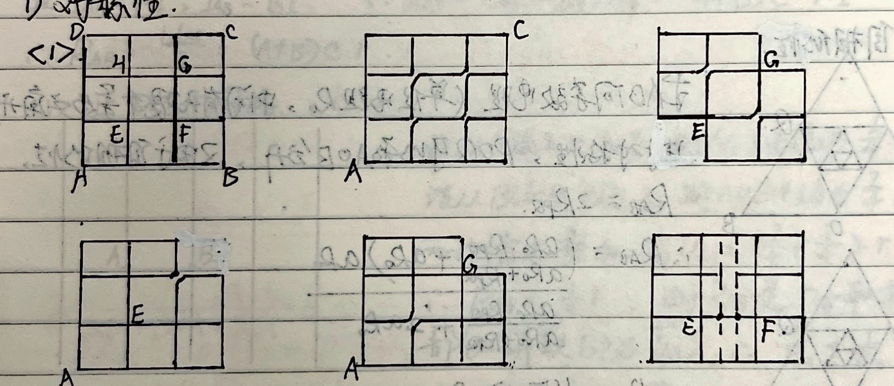
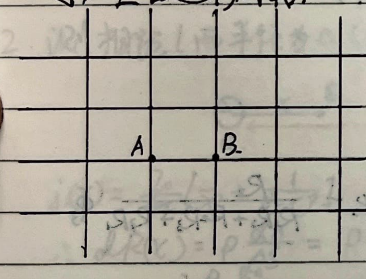
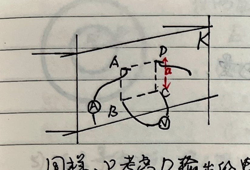
1) Symmetry:

<1> Folding symmetry in grids:

<2> Ladder network:

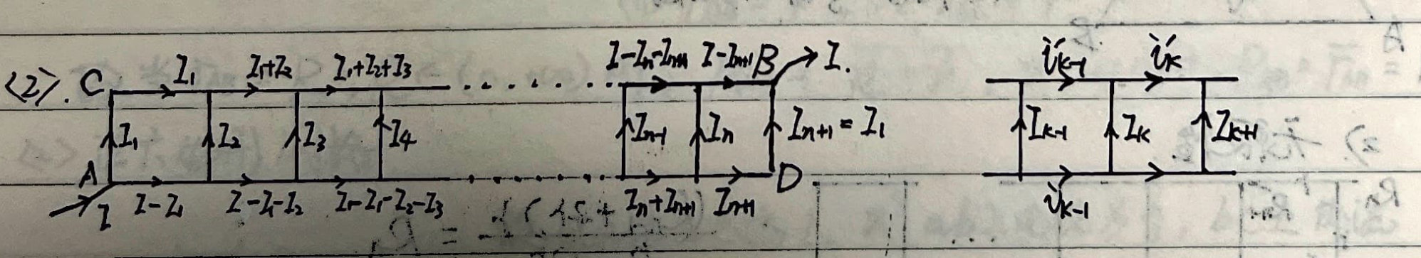$$ U_{CB} = U_{AD} = [I_1 + (I_1+I_2) + (I_1+I_2+I_3) + \dots + (I-I_{n+1})] R $$ $$ = [(I-I_1) + (I-I_1-I_2) + \dots + I_{n+1}] R $$ $$ \therefore 2U_{CB} = n I R $$

Also, from the loop equations:

$$ \begin{cases} I_k R + i_k' R = i_{k-1}' R + I_k R \\ I_k R + i_k'' R = i_k' R + I_{k+1} R \end{cases} \implies \begin{cases} i_{k-1}' + I_k = i_k'' \\ i_k' = I_k + i_k'' \end{cases} $$

Solving this yields $4I_k = I_{k+1} + I_{k-1}$. Transforming this recurrence relation:

$$ I_{n+1} - (2-\sqrt{3})I_n = (2+\sqrt{3}) [I_n - (2-\sqrt{3})I_{n-1}] $$

Because of conjugate symmetry, $I_{n+1} = I_1$, $I_n = I_2$. Solving gives:

$$ I_2 = \frac{(2+\sqrt{3})^{n-2} - (2-\sqrt{3})^{n-2}}{(2+\sqrt{3})^{n-1} - (2-\sqrt{3})^{n-1} + (2-\sqrt{3}) - (2+\sqrt{3})} I_1 $$

And from the first segment: $2I_1 R = (I - I_1)R \implies I_2 = 3I_1 - I$. Combining these yields $I_1$ in terms of $I$.

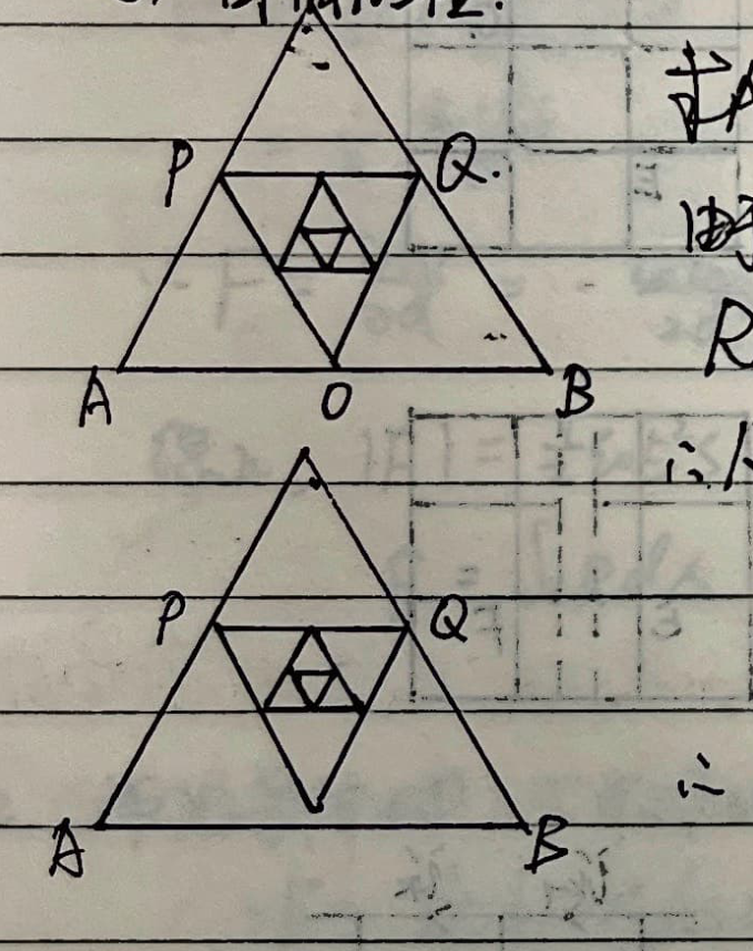
$$ \therefore U_{AB} = I_1 R + U_{BC} $$ $$ R_{AB} = \frac{U_{AB}}{I} = \left\{ \frac{n}{2} + \left[ 3 - \frac{(2+\sqrt{3})^{n-2} - (2-\sqrt{3})^{n-2}}{(2+\sqrt{3})^{n-1} - (2-\sqrt{3})^{n-1} - 2\sqrt{3}} \right]^{-1} \right\} R $$

<3> Self-similarity:

Find the equivalent resistance between A and B (unit resistance $R_0$, with infinite equilateral triangles inside).

By symmetry, POQ can be separated from AOB, and due to self-similarity:

$$ R_{AB} = 2 R_{PQ} $$ $$ \therefore R_{AB} = \frac{ \frac{aR_0 \cdot R_{PQ}}{aR_0 + R_{PQ}} + aR_0 }{ \frac{aR_0 \cdot R_{PQ}}{aR_0 + R_{PQ}} + 2aR_0 } a R_0 $$

Solving this equation gives:

$$ \therefore R_{AB} = \frac{1}{3}(\sqrt{7}-1) a R_0 $$

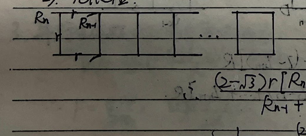
2) Infinity:

$$ \frac{(R_{n-1} + 2r) r}{R_{n-1} + 3r} = R_n $$ $$ \frac{(2-\sqrt{3})r[R_{n-1} + (1-\sqrt{3})r]}{R_{n-1} + 3r} = R_n + (1-\sqrt{3})r $$

Rearranging the terms gives:

$$ \frac{1}{R_n + (1-\sqrt{3})r} - \frac{2+\sqrt{3}}{R_{n-1} + (1-\sqrt{3})r} = \frac{1}{(2-\sqrt{3})r} = 2+\sqrt{3} $$

Solving the recurrence relation:

$$ R_n = -\frac{1}{2\sqrt{3}}r + \left[ \frac{1}{R_1 + (1-\sqrt{3})r} + \frac{1}{2\sqrt{3}r} \right] (7+4\sqrt{3})^{n-1} + (\sqrt{3}-1)r $$

When $n \to \infty$:

$$ R_\infty = (\sqrt{3}-1)r $$

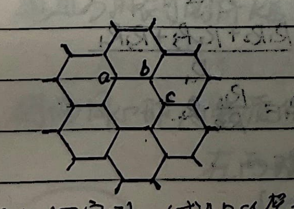
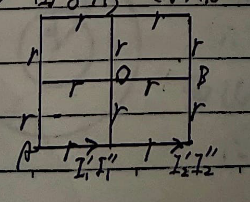
3) Current Superposition Method:

Assume a current $I$ flows into one node, calculate the current $I_{AB}$ flowing through the target branch AB. Assume a current $I$ flows out of the other node, calculate the current $I_{AB}'$ in AB. If $r_{AB}$ is the resistance of the wire connecting A and B ($r_{AB} = c \cdot r$), and $I_{AB} = A \cdot I$, $I_{AB}' = B \cdot I$:

$$ \therefore U_{AB} = (I_{AB} + I_{AB}') r_{AB} = (A+B) c \cdot r \cdot I \implies R_{AB} = \frac{U_{AB}}{I} = (A+B) c \cdot r $$

<1> Square Grid:

Assume $I$ flows into A, current on AB is $\frac{I}{4}$. Assume $I$ flows out of B, current on AB is $\frac{I}{4}$.

Superposing both cases: $U_{AB} = (\frac{I}{4} + \frac{I}{4}) \cdot r \implies R_{AB} = \frac{1}{2} r$.

Since $R_{AB}$ is the parallel combination of $r_{AB}$ and the rest of the grid (denoted $\overline{r_{AB}}$):

$$ \frac{1}{r_{AB}} + \frac{1}{\overline{r_{AB}}} = \frac{2}{r} $$

Since $r_{AB} = r$, we get $\overline{r_{AB}} = r$.

Thus, when $r_{AB} = R, R \in (0, +\infty)$, $R_{AB} = \frac{Rr}{R+r}$; when $r_{AB} = 0$, $R_{AB} = \overline{r_{AB}} = r$.

<2> Hexagonal Grid:

Assume $I$ flows into a, current on ab is $\frac{I}{3}$, current on bc is $\frac{I}{6}$.

Assume $I$ flows out of c, current on bc is $\frac{I}{6}$, current on ab is $\frac{I}{3}$.

Superposing both cases: $U_{ac} = (\frac{I}{3} + \frac{I}{6})r + (\frac{I}{6} + \frac{I}{3})r = I r \implies R_{ac} = r$.

<3> Cross Grid / "" Shape:

Find equivalent resistance between A and B.

Assume $I$ flows into A and out of O. Solving yields $I_1' = \frac{7}{24} I, I_2' = \frac{1}{8} I$.

Assume $I$ flows into O and out of B. Solving yields $I_1'' = \frac{7}{24} I, I_2'' = \frac{5}{24} I$.

$$ \therefore I_1 = \frac{7}{24}I + \frac{7}{24}I = \frac{14}{24} I, \quad I_2 = \frac{1}{8}I + \frac{5}{24}I = \frac{1}{3} I $$ $$ \therefore U_{AB} = I_1 r + I_2 \cdot 2r \implies R_{AB} = \frac{U_{AB}}{I} = \left(\frac{14}{24} + \frac{2}{3}\right)r = \frac{30}{24} r = \frac{5}{4} r $$

(Note: The manuscript calculation is approximated as $\frac{29}{24} r$ based on the diagram labels).

4) Y-$\Delta$ Transform (Y-$\Delta$ ):

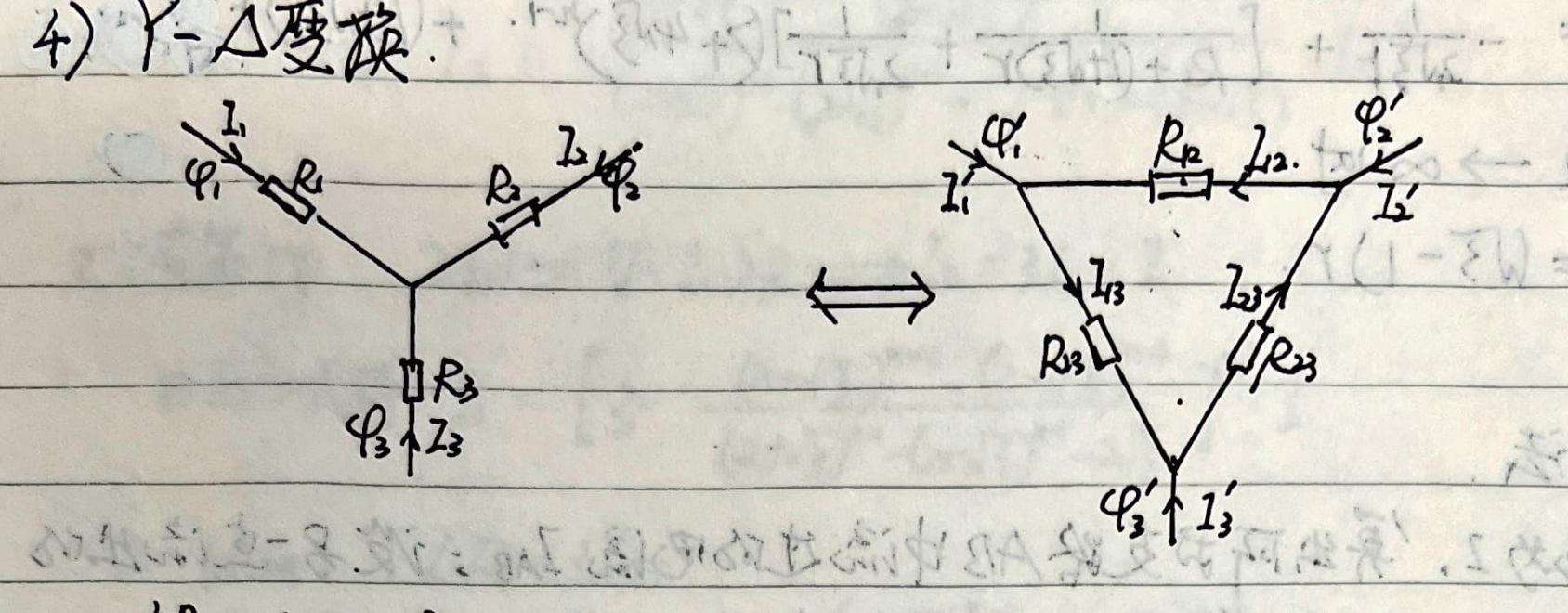
Equivalence implies: $I_1 = I_1', I_2 = I_2', I_3 = I_3'$ and $\varphi_1 = \varphi_1', \varphi_2 = \varphi_2', \varphi_3 = \varphi_3'$.

In the Y-shape (using node voltage method and Kirchhoff's current law):

$$ \begin{cases} \varphi_1 - I_1 R_1 + I_3 R_3 = \varphi_3 \\ \varphi_1 - I_1 R_1 + I_2 R_2 = \varphi_2 \\ I_1 + I_2 + I_3 = 0 \end{cases} $$

In the $\Delta$-shape:

$$ \begin{cases} \varphi_1' - I_{13} R_{13} = \varphi_3' \\ \varphi_1' + I_{12} R_{12} = \varphi_2' \\ I_1' = I_{13} - I_{12} \end{cases} $$

From the Y-shape, we can express $I_1$ in terms of the potentials:

$$ I_1 = \frac{R_2+R_3}{R_1 R_2 + R_2 R_3 + R_3 R_1} \varphi_1 - \frac{R_3}{R_1 R_2 + R_2 R_3 + R_3 R_1} \varphi_2 - \frac{R_2}{R_1 R_2 + R_2 R_3 + R_3 R_1} \varphi_3 $$

From the $\Delta$-shape:

$$ I_1' = \left(\frac{1}{R_{31}} + \frac{1}{R_{12}}\right) \varphi_1' - \frac{1}{R_{12}} \varphi_2' - \frac{1}{R_{31}} \varphi_3' $$

Comparing the coefficients of the potentials, we get:

$$ R_{12} = \frac{R_1 R_2 + R_2 R_3 + R_3 R_1}{R_3}, \quad R_{31} = \frac{R_1 R_2 + R_2 R_3 + R_3 R_1}{R_2}, \quad R_{23} = \frac{R_1 R_2 + R_2 R_3 + R_3 R_1}{R_1} $$

By solving the reverse transformation from $\Delta$ to Y:

$$ R_1 = \frac{R_{12} R_{31}}{R_{12} + R_{23} + R_{31}}, \quad R_2 = \frac{R_{23} R_{12}}{R_{12} + R_{23} + R_{31}}, \quad R_3 = \frac{R_{23} R_{31}}{R_{12} + R_{23} + R_{31}} $$

Special Topic: Measuring Resistivity

1. Measuring the resistivity of an infinite medium:

Draw a square ABCD of side $a$ on the surface. Inject current $I_0$ at A, and extract the same current $I_0$ at D.

For the injected current at A, the current density is $j = \frac{I_0}{2\pi r^2} \implies E = \frac{j}{\sigma} = \frac{I_0 \rho}{2\pi r^2}$.

$$ \therefore \varphi = -\int E dr = \frac{I_0 \rho}{2\pi r} $$ $$ \therefore U_{BC} = \frac{I_0 \rho}{2\pi a} - \frac{I_0 \rho}{2\pi (\sqrt{2}a)} = \frac{(2-\sqrt{2})I_0 \rho}{4\pi a} $$

Similarly, considering only the extracted current at D, $U_{BC}' = \frac{(2-\sqrt{2})I_0 \rho}{4\pi a}$. By superposition:

$$ U_0 = U_{BC} + U_{BC}' = \frac{(2-\sqrt{2})I_0 \rho}{2\pi a} $$ $$ \therefore \rho = \frac{2\pi a}{(2-\sqrt{2})} \frac{U_0}{I_0} = (2+\sqrt{2})\pi a \frac{U_0}{I_0} $$

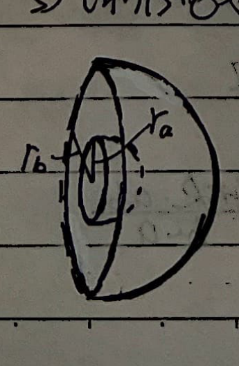
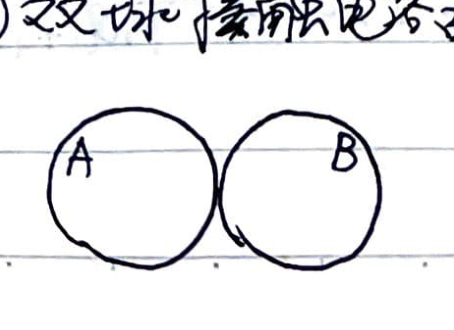
2. Measuring the resistivity of space where two metal spheres of radius $a$ are separated by distance $l \gg a$ (Multimeter reading is R):

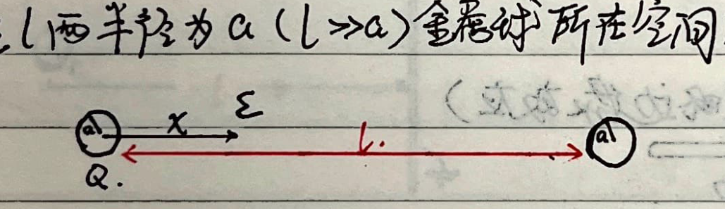
The current density at a point $x$ between the spheres is:

$$ j(x) = \frac{I_0}{4\pi} \left[ \frac{1}{x^2} + \frac{1}{(l-x)^2} \right] \quad (a < x < l-a) $$ $$ \therefore dR(x) = \rho \frac{dx}{S} = \frac{\rho dx}{I_0} j(x) = \frac{\rho dx}{I_0} \frac{I_0}{4\pi} \left[ \frac{1}{x^2} + \frac{1}{(l-x)^2} \right] = \frac{\rho}{4\pi} \left[ \frac{1}{x^2} + \frac{1}{(l-x)^2} \right] dx $$ $$ \therefore R = \frac{\rho}{4\pi} \int_a^{l-a} \left[ \frac{1}{x^2} + \frac{1}{(l-x)^2} \right] dx = \frac{\rho}{4\pi} \cdot 2 \left( \frac{1}{a} - \frac{1}{l-a} \right) = \frac{\rho}{2\pi} \left( \frac{1}{a} - \frac{1}{l-a} \right) $$

The multimeter measures this total resistance $R_{\text{total}}$.

$$ \therefore \rho = \frac{2\pi R_{\text{total}} a (l-a)}{l-2a} $$

When $l \to \infty$, $\rho = 2\pi R_{\text{total}} a$.

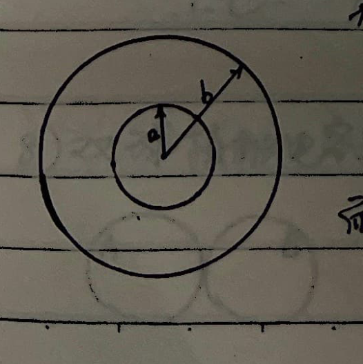
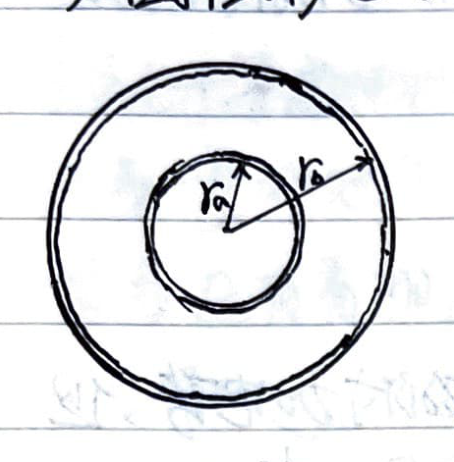
3. Measuring the resistivity of the substance between two concentric spheres:

Take a Gaussian surface of radius $r$ between the two spherical surfaces:

$$ \oint E dS = E \cdot 4\pi r^2 = \frac{Q}{\varepsilon_1} = \rho \oint j dS = \rho I $$ $$ \therefore Q = \varepsilon_1 \rho I $$

And $U_{ab} = \frac{Q}{4\pi\varepsilon_1} \left(\frac{1}{a} - \frac{1}{b}\right) = I R$. Substituting $Q$:

$$ \frac{\varepsilon_1 \rho I}{\varepsilon_1} = \frac{4\pi R a b}{b - a} \cdot I $$ $$ \therefore \rho = \frac{4\pi R a b}{b - a} $$

2. Capacitance

① Definition: $C = \frac{Q}{U}$

$U$: potential difference between two plates.
$Q$: charge passing through the wire after connecting the two plates.

② Series and Parallel Circuits:

Series: $\frac{1}{C_{\text{total}}} = \frac{U_{\text{total}}}{Q} = \sum \frac{U_i}{Q} = \sum \frac{1}{C_i}$
Parallel: $C_{\text{total}} = \frac{Q_{\text{total}}}{U} = \sum \frac{Q_i}{U} = \sum C_i$

③ Energy of a capacitor:

$$ W = \int q dU = \int_0^Q q \frac{dq}{C} = \frac{1}{2} \frac{Q^2}{C} = \frac{1}{2} \frac{Q^2}{\varepsilon S} d = \frac{1}{2} \left(\frac{Q}{\varepsilon S}\right)^2 \varepsilon S d = \frac{1}{2} E^2 \varepsilon S d = \frac{1}{2} \varepsilon E^2 \cdot V $$

Energy density: $\omega = \frac{dW}{dV} = \frac{1}{2} \varepsilon E^2$

④ Typical capacitor capacitance:

1) Parallel plate capacitor (ignoring edge effects):

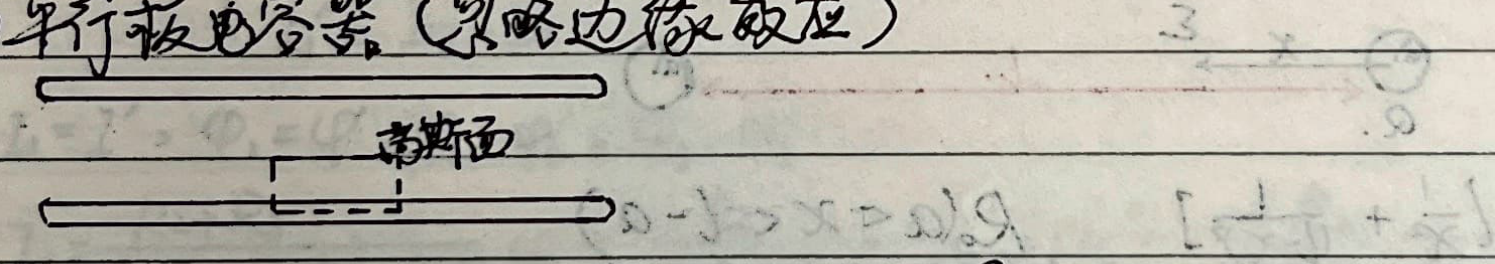$$ E_{\Delta S} = \frac{\sigma \Delta S}{\varepsilon_0} \implies E = \frac{Q}{\varepsilon_0 S} \implies U = E d = \frac{Q d}{\varepsilon_0 S} $$ $$ \therefore C = \frac{Q}{U} = \frac{\varepsilon_0 S}{d} $$

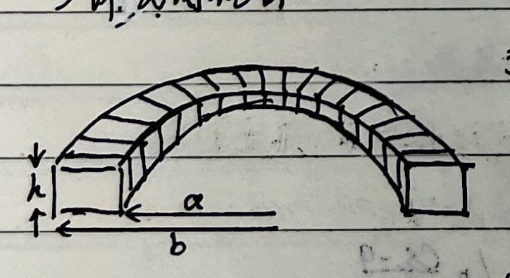
2) Tilted parallel plate capacitor ($h \ll d$):

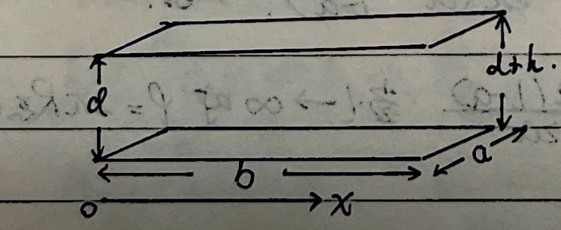
Treat the whole capacitor as an infinite number of $dC$ elements in parallel.

$$ dC = \frac{\varepsilon_0 a dx}{d + \frac{h}{b}x} $$ $$ \therefore C = \int_0^b \frac{\varepsilon_0 a dx}{d + \frac{h}{b}x} = \frac{\varepsilon_0 a b}{h} \ln\left(1 + \frac{h}{d}\right) $$

3) Spherical capacitor:

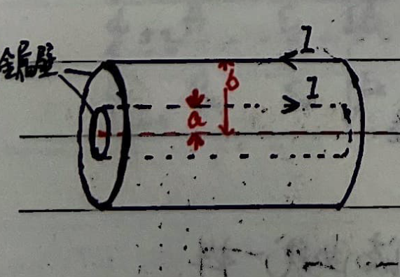
$$ \varphi_A = \frac{1}{4\pi\varepsilon_0}\left(\frac{q}{r_a} + \frac{-q}{r_b}\right) $$ $$ \varphi_B = \frac{1}{4\pi\varepsilon_0}\left(\frac{q}{r_b} + \frac{-q}{r_b}\right) $$ $$ \therefore U_{AB} = \varphi_A - \varphi_B = \frac{q}{4\pi\varepsilon_0}\left(\frac{1}{r_a} - \frac{1}{r_b}\right) $$ $$ \therefore C = \frac{q}{U_{AB}} = \frac{4\pi\varepsilon_0 r_a r_b}{r_b - r_a} $$

4) Cylindrical capacitor (length $L$):

Take a cylindrical Gaussian surface of radius $r$ between the two cylinders:

$$ E \cdot 2\pi r \cdot L = \frac{q}{\varepsilon_0} \implies E = \frac{q}{2\pi\varepsilon_0 r L} $$ $$ \therefore U_{ab} = \int_{r_a}^{r_b} E dr = \frac{q}{2\pi\varepsilon_0 L} \int_{r_a}^{r_b} \frac{dr}{r} = \frac{q}{2\pi\varepsilon_0 L} \ln\left(\frac{r_b}{r_a}\right) $$ $$ \therefore C = \frac{q}{U_{ab}} = \frac{2\pi\varepsilon_0 L}{\ln\frac{r_b}{r_a}} $$

When $r_b - r_a \ll r_a, r_b$, $C \approx \frac{2\pi\varepsilon_0 r_a L}{r_b - r_a}$.

5) Isolated conducting sphere:

Treat infinity as the other plate.

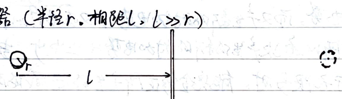
$$ \because \varphi_\infty = 0, \quad \varphi_R = \frac{Q}{4\pi\varepsilon_0 R} $$ $$ \therefore U = \frac{Q}{4\pi\varepsilon_0 R} \implies C = \frac{Q}{U} = 4\pi\varepsilon_0 R $$

6) Sphere-plate capacitor (radius $r$, distance $L$, $L \gg r$):

Make an image of the metal sphere on the right side of the metal plate, remove the plate, in this two-sphere system:

$$ U_{ab} = \frac{kq}{r} - \left(\frac{-kq}{r}\right) = \frac{2kq}{r} = \frac{q}{2\pi\varepsilon_0 r} $$ $$ \therefore C = \frac{q}{U_{ab}} = 2\pi\varepsilon_0 r $$

This two-sphere system is exactly equivalent to two sphere-plate capacitors in series, so the sphere-plate capacitance is $C' = 4\pi\varepsilon_0 r$.

7) Two-sphere connected capacitor (radii $r_a, r_b$, distance $L$, $L \gg r_a, r_b$):

Because the two spheres are connected by a wire:

$$ \varphi_a = \varphi_b \implies \frac{q_1}{r_a} = \frac{q_2}{r_b} $$

Taking infinity as the other plate, $\varphi_\infty = 0$:

$$ \therefore U = \varphi_a - \varphi_\infty = \frac{kq_1}{r_a} $$ $$ \therefore C = \frac{q_1+q_2}{U} = \frac{q_1 + \frac{r_b}{r_a}q_1}{\frac{kq_1}{r_a}} = 4\pi\varepsilon_0(r_a+r_b) $$

8) Two-sphere contacting capacitor (radius $R$, distance $2R$):

Assume the system potential is $U_0$. Imagine the charge of both spheres stays at their centers; ignoring mutual induction, the potential of both spheres is $U_0$, and $q_1 = 4\pi\varepsilon_0 R U_0$.

Because mutual induction will make the potential of the two spheres higher than $U_0$, to eliminate this additional potential, an image charge needs to be added inside each sphere:

$$ q_2 = -\frac{R}{2R} q_1 = -\frac{1}{2} q_1, \quad x_2 = \frac{R^2}{2R} = \frac{1}{2} R $$

This way, each internal image charge can eliminate the other's additional potential, but generates its own new additional potential, which requires new image charges to cancel:

$$ q_3 = -\frac{R}{2R-x_2} q_2 = \frac{1}{3} q_1, \quad x_3 = \frac{R^2}{2R-x_2} = \frac{2}{3} R $$

And so on. Each newly added image charge cancels the previously generated additional potential, while generating a new one. Because $|q_{n+1}| < |q_n|$, each new additional potential is smaller. As the number of image charges approaches infinity, it completely corrects the diminishing additional potentials, restoring the system potential to $U_0$.

$$ \implies \begin{cases} q_n = \frac{(-1)^{n-1}}{n} q_1 \\ x_n = \frac{n-1}{n} R \end{cases} $$

The total charge on the conducting spheres is equal to $q_1$ plus the total charge of all image charges:

$$ Q_{\text{total}} = 2(q_1 + q_2 + \dots) = 2 q_1 \left(1 - \frac{1}{2} + \frac{1}{3} - \frac{1}{4} + \dots\right) = 8\pi\varepsilon_0 R U_0 \ln 2 $$ $$ \therefore C = \frac{Q_{\text{total}}}{U_0} = 8\pi\varepsilon_0 R \ln 2 $$

9) Leaky capacitor:

Because voltage $U$ is applied across the plates:

$$ I = \frac{U}{\rho_1 \frac{d_1}{S} + \rho_2 \frac{d_2}{S}} = \frac{U S}{\rho_1 d_1 + \rho_2 d_2} $$ $$ \therefore E_1 = \rho_1 \frac{I}{S} = \frac{\rho_1 U}{\rho_1 d_1 + \rho_2 d_2}, \quad E_2 = \rho_2 \frac{I}{S} = \frac{\rho_2 U}{\rho_1 d_1 + \rho_2 d_2} $$

Also, $C_1 = \frac{\varepsilon_0 \varepsilon_1 S}{d_1}$ and $C_2 = \frac{\varepsilon_0 \varepsilon_2 S}{d_2}$:

$$ \therefore q_1 = E_1 d_1 C_1 = \frac{\rho_1 \varepsilon_0 \varepsilon_1 S U}{\rho_1 d_1 + \rho_2 d_2}, \quad q_2 = E_2 d_2 C_2 = \frac{\rho_2 \varepsilon_0 \varepsilon_2 S U}{\rho_1 d_1 + \rho_2 d_2} $$

Therefore, the surface charge density at the interface of the two dielectrics is:

$$ \sigma = \frac{\varepsilon_0 (\rho_1 \varepsilon_1 - \rho_2 \varepsilon_2) U}{\rho_1 d_1 + \rho_2 d_2} $$

⑤ Equivalent Capacitance:

Similar to equivalent resistance, it has symmetry and infinite series solutions. Also, because in a two-terminal passive circuit, $R$ and $\frac{1}{C}$ have the same mathematical status:

Series: $R = \sum R_i, C = (\sum \frac{1}{C_i})^{-1}$
Parallel: $R = (\sum \frac{1}{R_i})^{-1}, C = \sum C_i$

Therefore, it has the opposite Y-$\Delta$ transform to $R$.

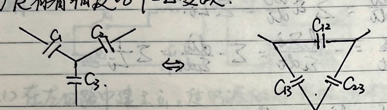$$ \begin{cases} C_{12} = \frac{C_1 C_2}{C_1 + C_2 + C_3} \\ C_{23} = \frac{C_2 C_3}{C_1 + C_2 + C_3} \\ C_{31} = \frac{C_3 C_1}{C_1 + C_2 + C_3} \end{cases} \iff \begin{cases} C_3 = \frac{C_{12} C_{23} + C_{12} C_{31} + C_{23} C_{31}}{C_{12}} \\ C_1 = \frac{C_{12} C_{23} + C_{12} C_{31} + C_{23} C_{31}}{C_{23}} \\ C_2 = \frac{C_{12} C_{23} + C_{12} C_{31} + C_{23} C_{31}}{C_{31}} \end{cases} $$

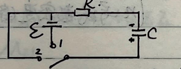
⑥ RC Circuits:

1) Charging:

$$ \mathcal{E} - i R - \frac{q}{C} = 0, \quad i = \frac{dq}{dt} $$ $$ \therefore \mathcal{E} = R \frac{dq}{dt} + \frac{q}{C} \implies dt = \frac{R C dq}{C\mathcal{E} - q} $$ $$ \therefore \int_0^t dt = -RC \int_0^q \frac{d(C\mathcal{E}-q)}{C\mathcal{E}-q} \implies t = -RC \ln \frac{C\mathcal{E}-q}{C\mathcal{E}} $$

Solving yields:

$$ q = C\mathcal{E} (1 - e^{-t/RC}), \quad i = \frac{dq}{dt} = \frac{\mathcal{E}}{R} e^{-t/RC} $$

2) Discharging:

$$ i R = \frac{q}{C}, \quad i = -\frac{dq}{dt} $$ $$ \therefore R \frac{dq}{dt} + \frac{q}{C} = 0 \implies dt = -RC \frac{dq}{q} $$ $$ \therefore t = -RC \ln \frac{q}{q_0} = -RC \ln \frac{q}{C\mathcal{E}} \implies q = C\mathcal{E} e^{-t/RC} $$ $$ i = -\frac{dq}{dt} = \frac{C\mathcal{E}}{RC} e^{-t/RC} = \frac{\mathcal{E}}{R} e^{-t/RC} $$

(Same current curve as charging.)

3. Inductance

① Definition:

$$ \mathcal{E}_L = -\frac{d\Psi}{dt} = -N \frac{d\Phi}{dt} = -\frac{d(LI)}{dt} = -L \frac{dI}{dt} $$ $$ \therefore L = -\mathcal{E}_L / \frac{dI}{dt} $$

② Series and Parallel:

Series: $L_{\text{total}} \frac{di}{dt} = \sum \mathcal{E}_{Li} = \sum L_i \frac{di}{dt} \implies L_{\text{total}} = \sum L_i$
Parallel: $\frac{1}{L_{\text{total}}} = -\frac{di_{\text{total}} / dt}{\mathcal{E}_L} = -\frac{d\sum i_i / dt}{\mathcal{E}_L} = \sum -\frac{di_i / dt}{\mathcal{E}_L} = \sum \frac{1}{L_i}$

③ Energy of inductance:

$$ W = \int \mathcal{E} i dt = \int -L \frac{di}{dt} i dt = \int -L i di = \frac{1}{2} L I^2 = \frac{1}{2} \mu_0 n^2 V I^2 $$

Also, from $B = \mu_0 n I$, eliminating $n I$ yields:

$$ W = \frac{B^2}{2\mu_0} V $$

Energy density: $\omega = \frac{dW}{dV} = \frac{B^2}{2\mu_0}$

④ Self-inductance:

1) Solenoid:

$$ \Psi = N \Phi = (l \cdot n) \cdot B S = l n \cdot \mu_0 n I S = L \cdot I $$ $$ \therefore L = \frac{\Psi}{I} = \mu_0 n^2 S \cdot l = \mu_0 n^2 V $$

Where $n$ is the turn density (turns/m).

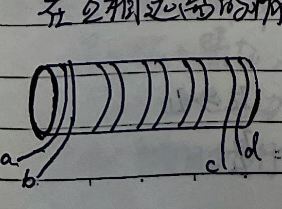
2) Toroidal solenoid:

Apply Ampere's law to the whole ring:

$$ B \cdot 2\pi r = \mu_0 N I \implies B = \frac{\mu_0 N I}{2\pi r} $$

Therefore, the flux linkage is:

$$ \Psi = N \cdot \int_a^b B \cdot h dr = N \frac{\mu_0 N I h}{2\pi} \ln\frac{b}{a} $$ $$ \therefore L = \frac{\mu_0 N^2 h}{2\pi} \ln\frac{b}{a} $$

3) Coaxial cable:

For a unit length of the cable ($l$):

$$ \Psi = \int_a^b B l dr = \frac{\mu_0 I l}{2\pi} \int_a^b \frac{dr}{r} = \frac{\mu_0 I l}{2\pi} \ln\frac{b}{a} $$ $$ \therefore L = \frac{\mu_0 l}{2\pi} \ln\frac{b}{a} $$

⑤ Mutual Inductance:

$$ \mathcal{E}_{21} = -M_{21} \frac{di_1}{dt}, \quad \mathcal{E}_{12} = -M_{12} \frac{di_2}{dt} $$

And $M_{12} = M_{21} = M$

Proof:

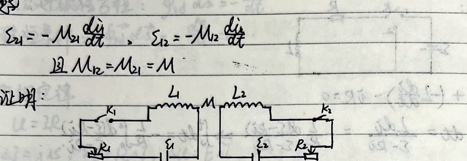
<1> Establish $i_1$ in the left circuit, the power source does work, and the energy stored in the magnetic field is $W_1 = \frac{1}{2} L_1 i_1^2$.

<2> Establish $i_2$ in the right circuit, the power source does work, storing energy $W_2 = \frac{1}{2} L_2 i_2^2$. But in this process, $L_1$ produces a back electromotive force. To keep $i_1$ constant, $\mathcal{E}_1$ must do additional work $W_{12} = -\int \mathcal{E}_{12} i_1 dt$:

$$ W_{12} = \int M_{12} i_1 \frac{di_2}{dt} dt = M_{12} i_1 \int_0^{I_2} di_2 = M_{12} I_1 I_2 $$

<3> After the above two processes, the system reaches the state where the currents are $I_1$ and $I_2$,

$$ W_{\text{total}} = W_1 + W_2 + W_{12} = \frac{1}{2} L_1 I_1^2 + \frac{1}{2} L_2 I_2^2 + M_{12} I_1 I_2 $$

<4> Starting by establishing $i_2$ in the right circuit first, reaching the same final state, the work done is similarly:

$$ W_{\text{total}} = \frac{1}{2} L_1 I_1^2 + \frac{1}{2} L_2 I_2^2 + M_{21} I_1 I_2 $$ $$ \therefore M_{12} = M_{21} $$

Mutual inductance between a long solenoid and a ring: (length $\gg$ radius, ring on the axis, axis perpendicular to the ring plane)

Assume the current in the solenoid is $i_1$, then the magnetic flux through the ring is $\Phi = B_1 \pi r^2 = \pi r^2 \mu_0 n i_1$

$$ \therefore M_{21} = \pi r^2 \mu_0 n $$ $$ \therefore M_{12} = M_{21} = \pi r^2 \mu_0 n $$

⑥ Equivalent Inductance:

When they are far apart, the calculation method is similar to equivalent resistance. Special case when they influence each other:

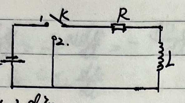
When $a-c$ or $b-d$ exists alone, the self-inductance is $L_0$.

$$ \begin{cases} a\text{ connected to }b, \text{circuit connected at }c, d\text{:} & L=0 \\ c\text{ connected to }b, \text{circuit connected at }a, d\text{:} & \Psi = (2 N_0) (\mu_0 2n_0 I) S, \ L = 4L_0 \\ a\text{ connected to }b, c\text{ connected to }d\text{:} & \Psi = N_0 \cdot (\mu_0 n_0 \frac{I}{2}) S \times 2, \ L = L_0 \end{cases} $$

⑦ RL Circuit:

1) Charging:

$$ \mathcal{E} + \left(-L \frac{di}{dt}\right) - iR = 0 $$ $$ \therefore dt = \frac{L di}{\mathcal{E} - i R} = -\frac{L}{R} \frac{d(\mathcal{E} - R i)}{\mathcal{E} - R i} \implies \int_0^t dt = -\frac{L}{R} \int_0^i \frac{d(\mathcal{E} - R i)}{\mathcal{E} - R i} $$ $$ \therefore t = -\frac{L}{R} \ln\left(\frac{\mathcal{E} - R i}{\mathcal{E}}\right) \implies \text{Solving yields } i = \frac{\mathcal{E}}{R}(1 - e^{-\frac{R}{L}t}) $$ $$ \therefore U_L = -L \frac{di}{dt} = -\mathcal{E} \cdot e^{-\frac{R}{L}t} $$

2) Discharging:

$$ -L \frac{di}{dt} - iR = 0 $$ $$ \therefore dt = -\frac{L}{R} \frac{di}{i} \implies \int_0^t dt = -\frac{L}{R} \int_{i_0}^i \frac{di}{i} $$ $$ \therefore t = -\frac{L}{R} \ln\frac{i}{i_0} \implies \text{Solving yields } i = i_0 e^{-\frac{R}{L}t} $$ $$ \therefore U_L = -iR = \mathcal{E} e^{-\frac{R}{L}t} $$

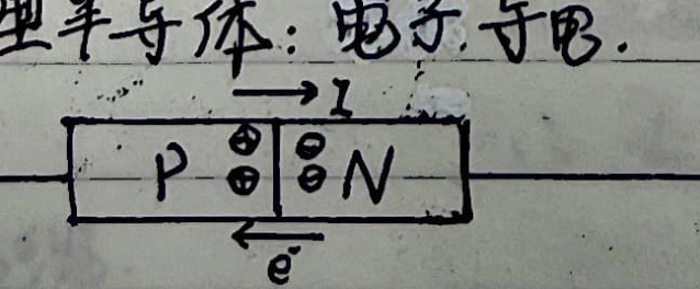
4. Semiconductors

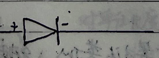
① Diode:

Ideal diode: Forward conducting $R=0$, reverse $R = \infty$.
Real diode: $i = I_s(e^{\frac{qU}{kT}} - 1)$.

$$ \begin{cases} P\text{-type semiconductor: hole conduction} \\ N\text{-type semiconductor: electron conduction} \end{cases} $$ PN junction

② Transistor:

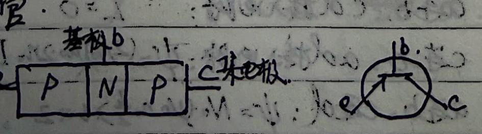
Emitter, Base, Collector.

$$ \begin{cases} I_e = I_b + I_c, \quad I_c \gg I_b \\ \beta = \frac{dI_c}{dI_b} \approx \frac{I_c}{I_b} \end{cases} $$